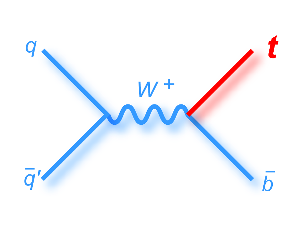
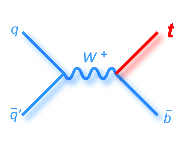
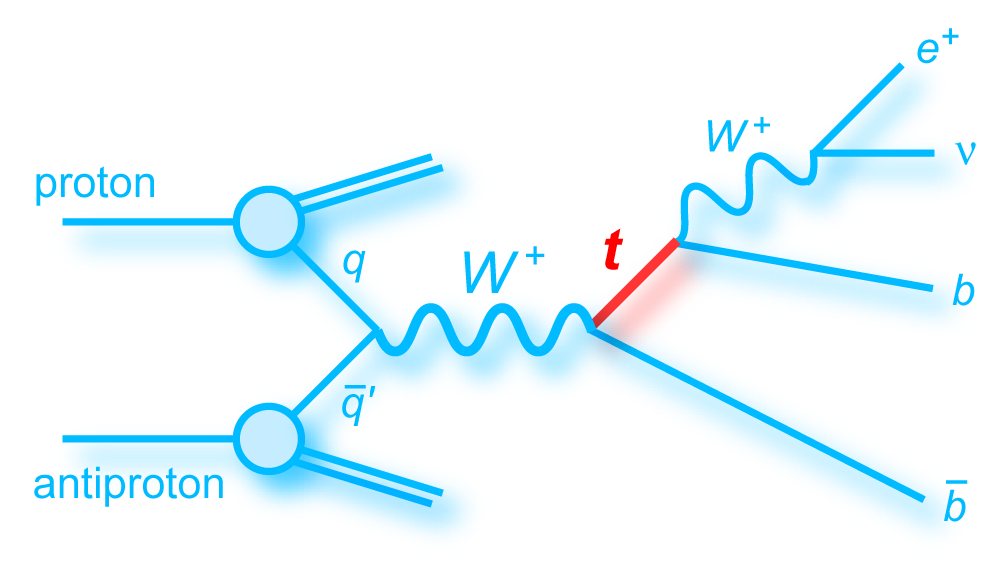
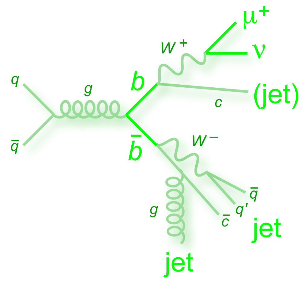
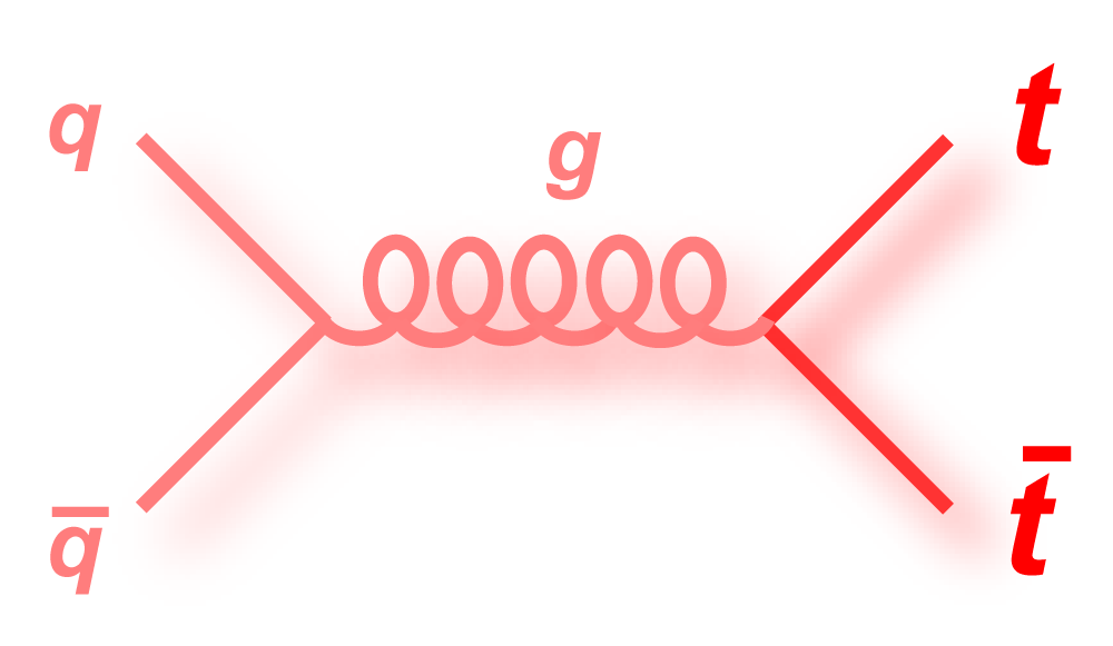
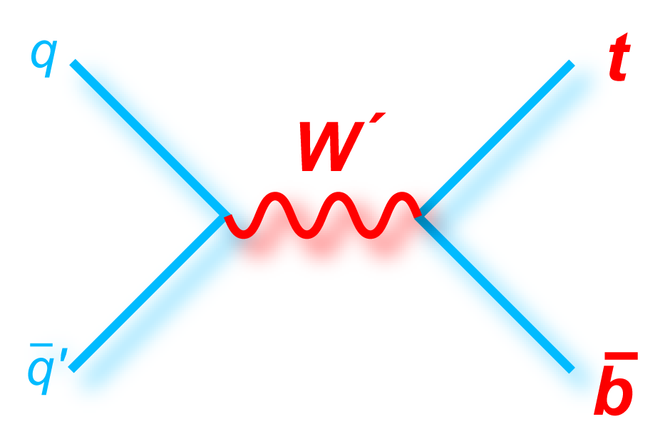
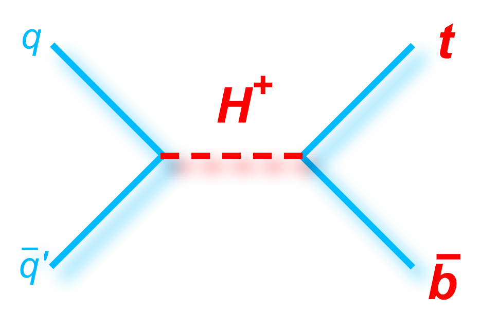
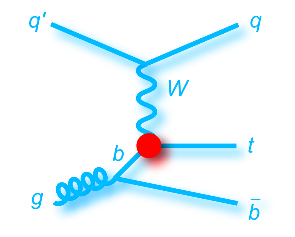
Observation of Single Top Quark Production by the DØ Collaboration

s-channel "tb"

Observation of Single Top Quark Production

The DØ Collaboration

March 2009

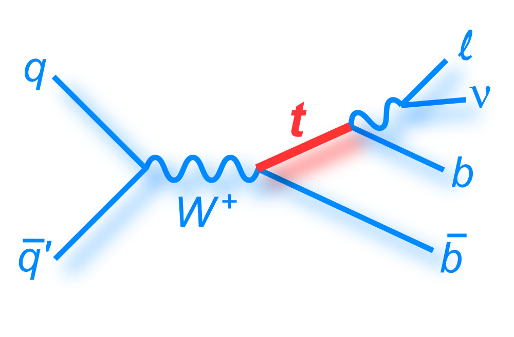
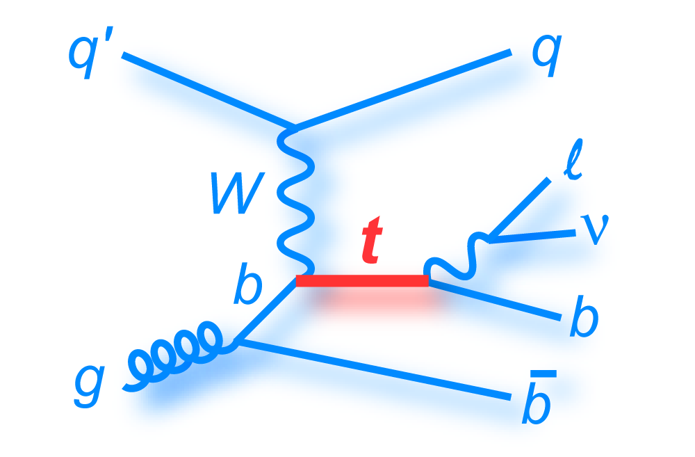
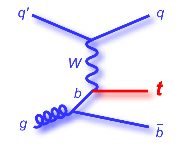
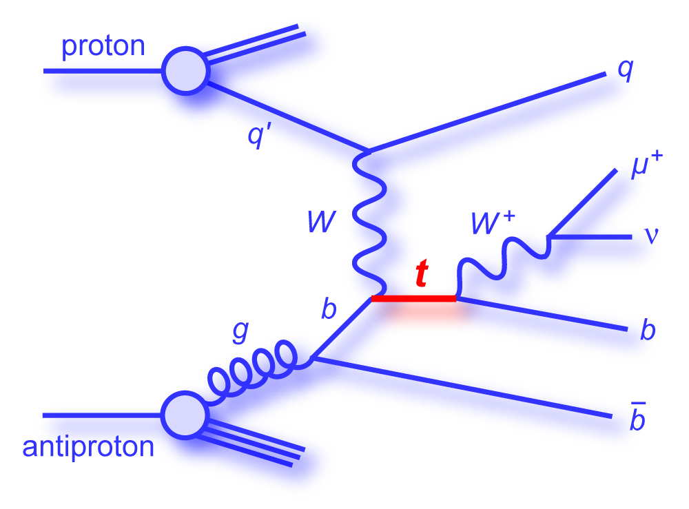
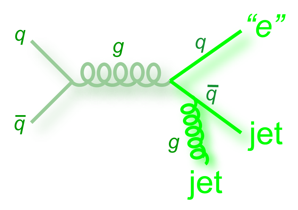
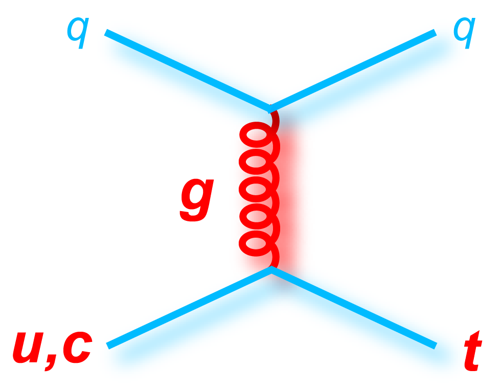
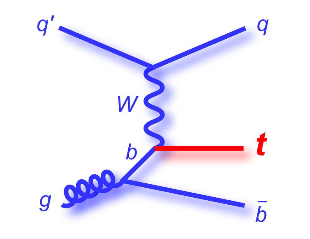t-channel "tqb"

Summary

On March 4, 2009, the DØ Collaboration submitted a paper to Physical Review Letters announcing the first observation of single top quark production. It was accepted for publication on July 20, and appeared in the journal on August 24, an "Editors' Suggestion" paper with a "Physics Synopsis" article.
"Observation of Single Top-Quark Production" arXiv:0903.0850 Phys. Rev. Lett. 103, 092001 (2009)
The search history:
• "Evidence for Production of Single Top Quarks"	March 2008	47 pages, TOPCITE=50+
• "Evidence for Production of Single Top Quarks and First Direct Measurement of \|V_tb\|"	December 2006	SPIRES TOPCITE=100+
• "Multivariate Searches for Single Top Quark Production with the DØ Detector"	April 2006	27 pages
• "Search for Single Top Quark Production in pp Collisions at √s = 1.96 TeV"	May 2005	SPIRES TOPCITE=50+
• "Search for Single Top Quark Production at DØ Using Neural Networks"	June 2001	SPIRES TOPCITE=50+
• "Search for Electroweak Production of Single Top Quarks in pp Collisions"	August 2000	SPIRES TOPCITE=50+

Contents

Abstract Event Selection Systematic Uncertainties Signal-Background Discrimination	Combination of Results Signal Plots CKM Matrix Element V_tb Observation Summary	Talks In the News More Images for Talks Contacts
(Click on a link to jump down the page)

Abstract

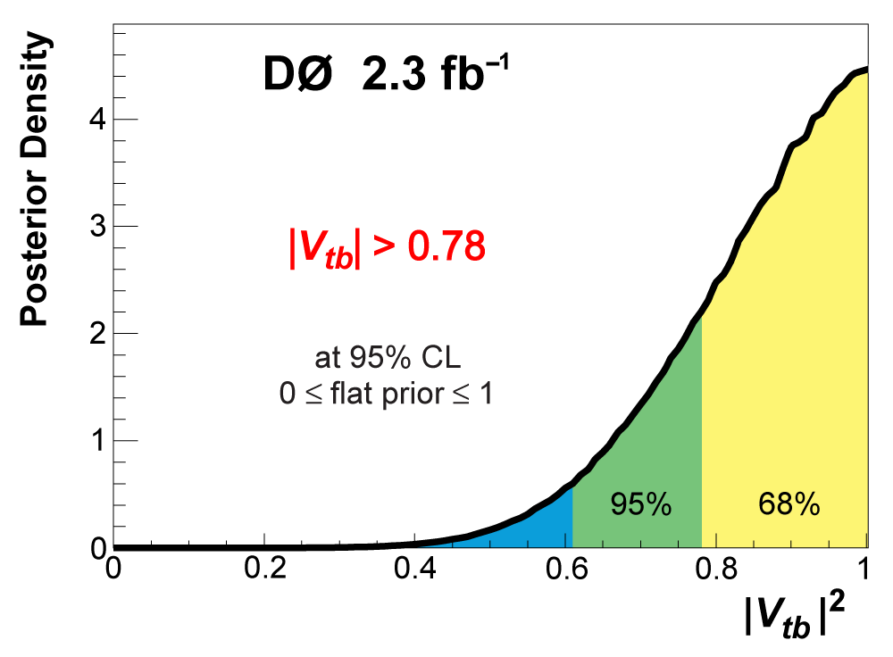
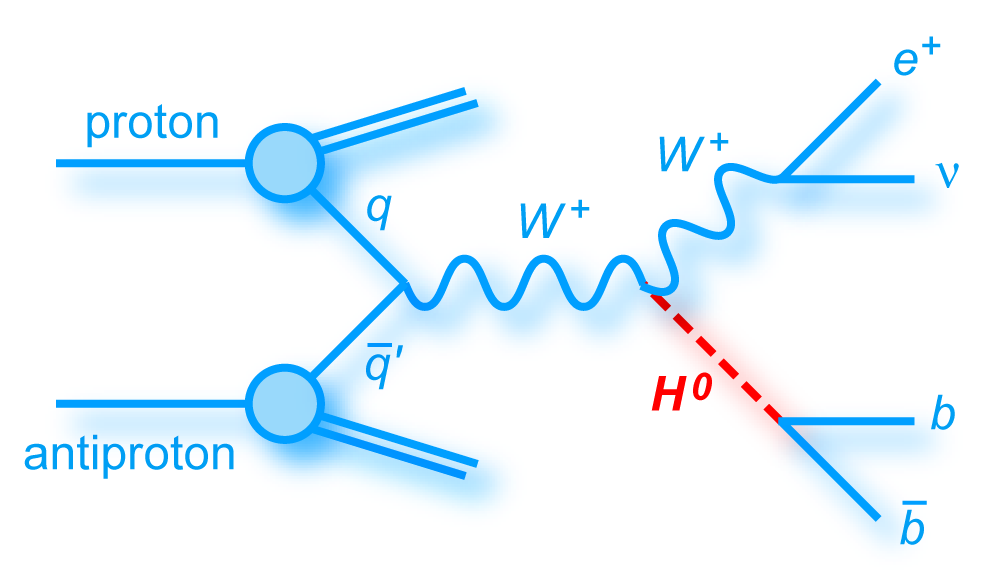
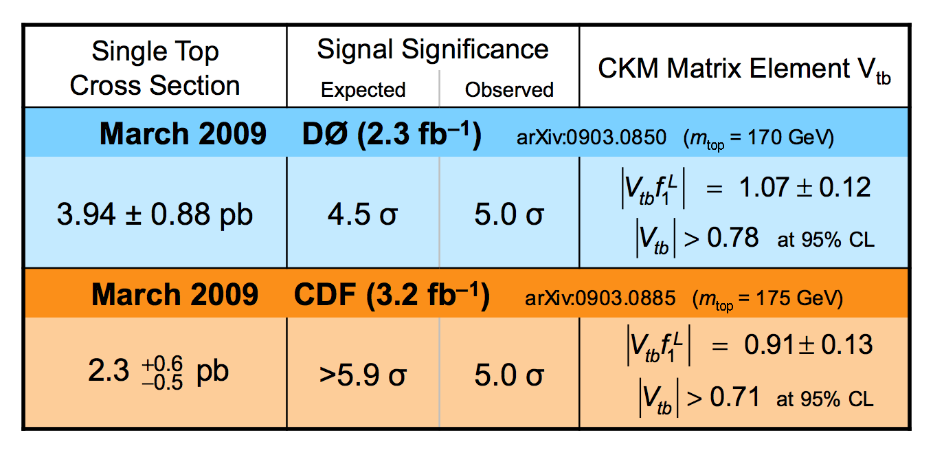
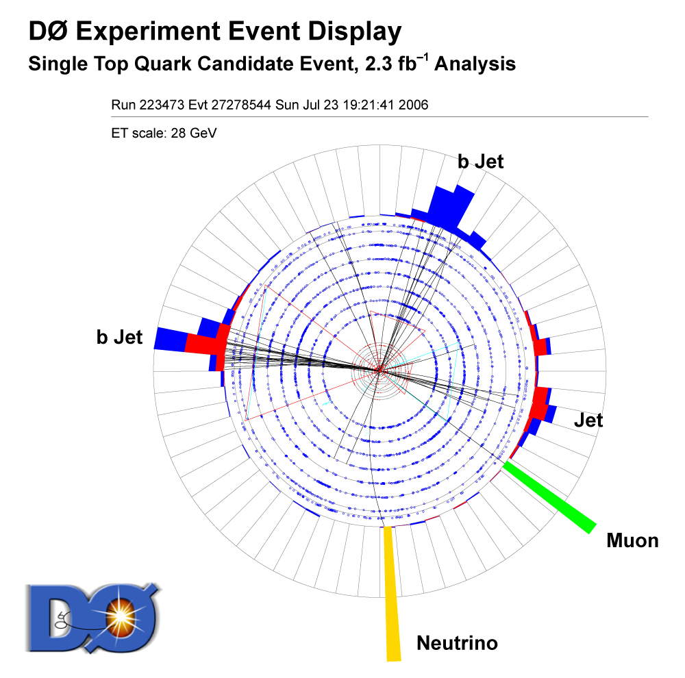
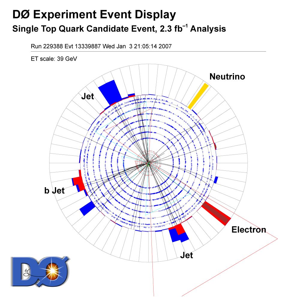
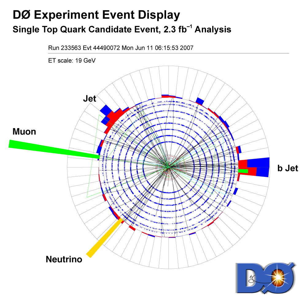
We present the results of a search for single top quark production in 2.3 fb^–1 of data at the Fermilab Tevatron proton-antiproton collider at 1.96 TeV center-of-mass energy. The events have an isolated high transverse-momentum electron or muon, together with missing transverse energy from the decay of a W boson from the top quark decay, and one or two bottom-quark jets. Some events have an additional light-quark jet. The predicted cross section for this process is 3.46 ± 1.8 pb for a top quark mass of 170 GeV. Our measurement is:

σ(pp → tb + X, tqb + X) = 3.94 ± 0.88 pb

where "tb" stands for tb + tb production, and "tq" stands for tqb + tqb production. The probability to measure a cross section at this value or higher in the absence of signal is 2.5 × 10^–7, corresponding to a 5.0 standard deviation significance for the presence of signal. This is considered an unlikely enough occurrence (1 in 4 million) that our measurement meets the standard to be called an observation of a new physics process. The results of our analysis are illustrated in the plot to the right.

We use the cross section measurement to make a direct measurement of the size of the CKM quark-mixing matrix element V_tb and find |V_tb f₁^L| = 1.07 ± 0.12, and when the strength of the left-handed scalar coupling f₁^L=1, we find |V_tb| > 0.78 at the 95% confidence level.

Cross section measurements in the 2.3ifb analysis

Parameters for the Measurement

The analysis is performed using a top quark mass of 170 GeV, which is close to the published world average value (171.2 GeV, Particle Data Book 2008 edition). The theoretical predictions for the cross sections of the two modes of single top quark production are 1.12 ± 0.04 pb for the s-channel tb mode and 2.34 ± 0.12 pb for the t-channel tqb mode (N. Kidonakis, Phys. Rev. D 74, 114012 (2006) with NNNLO-NLO matching, for m_top = 170 GeV and MRST2004 NNLO parton distribution functions). We do not use these values in the tb+tqb cross section measurement directly, but we assume the SM ratio of the processes, 1.12 : 2.34 = 1 : 2.1 when measuring the signal acceptance, selecting events used to train the BDT and BNN discriminants, and generating pseudo-datasets for the linearity tests.

Event Selection

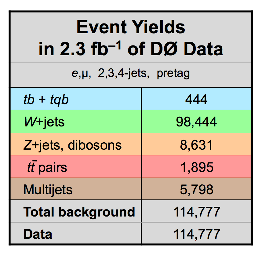
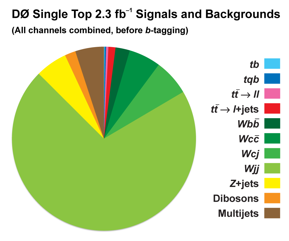
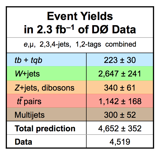
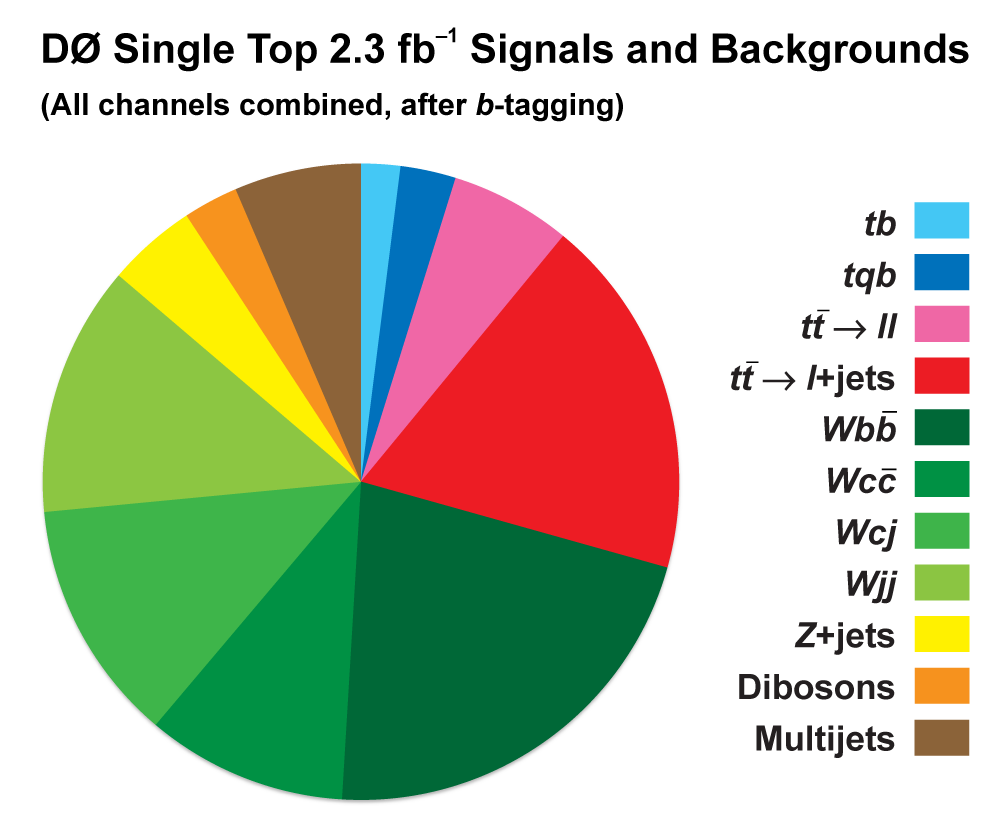
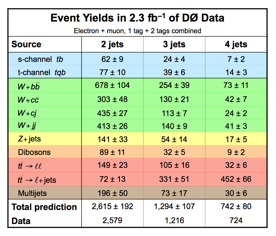
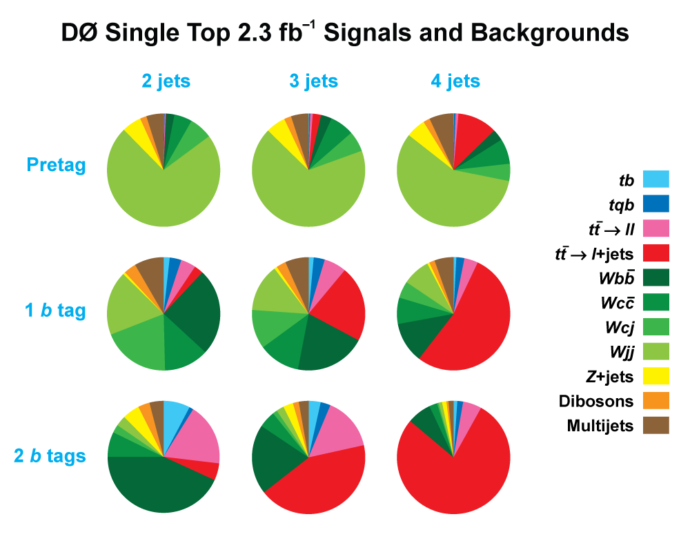
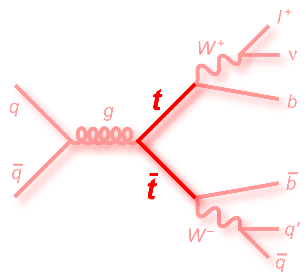
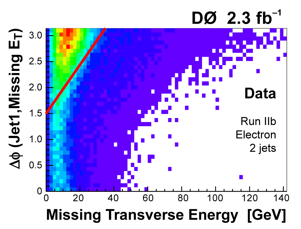
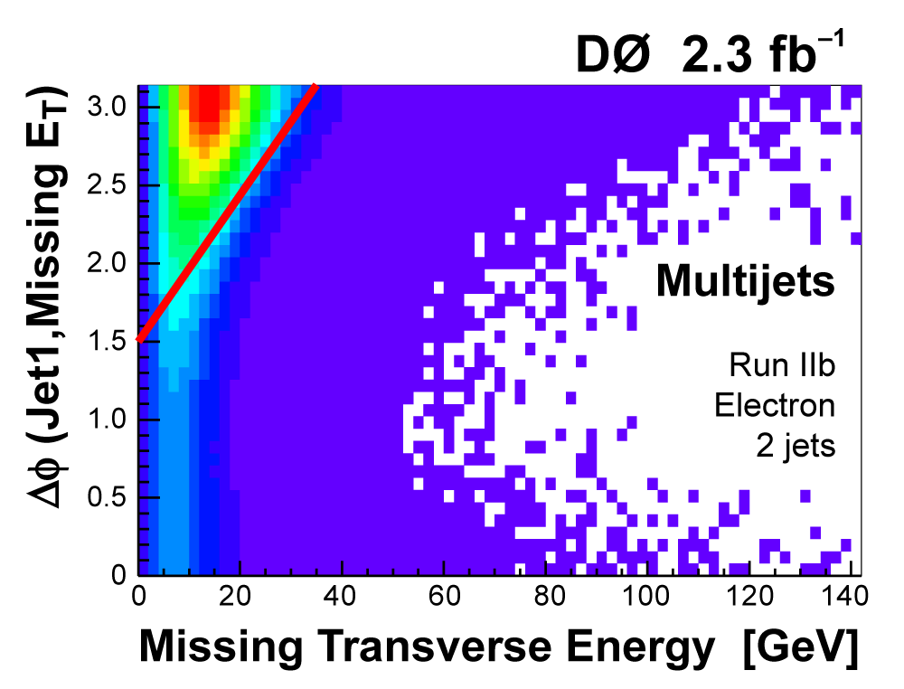
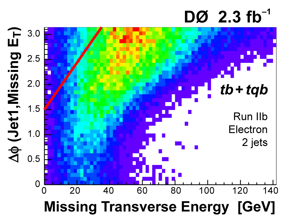
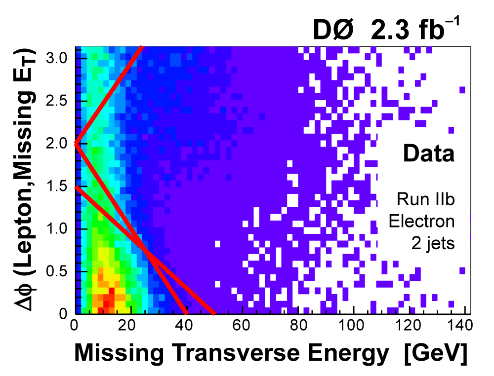
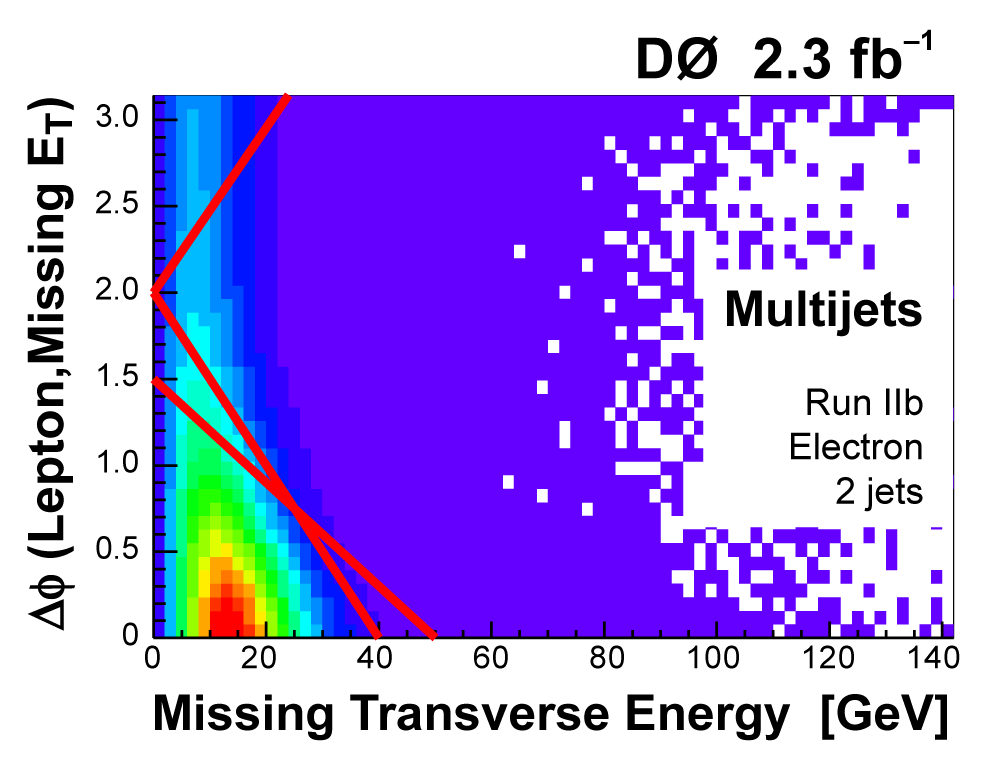
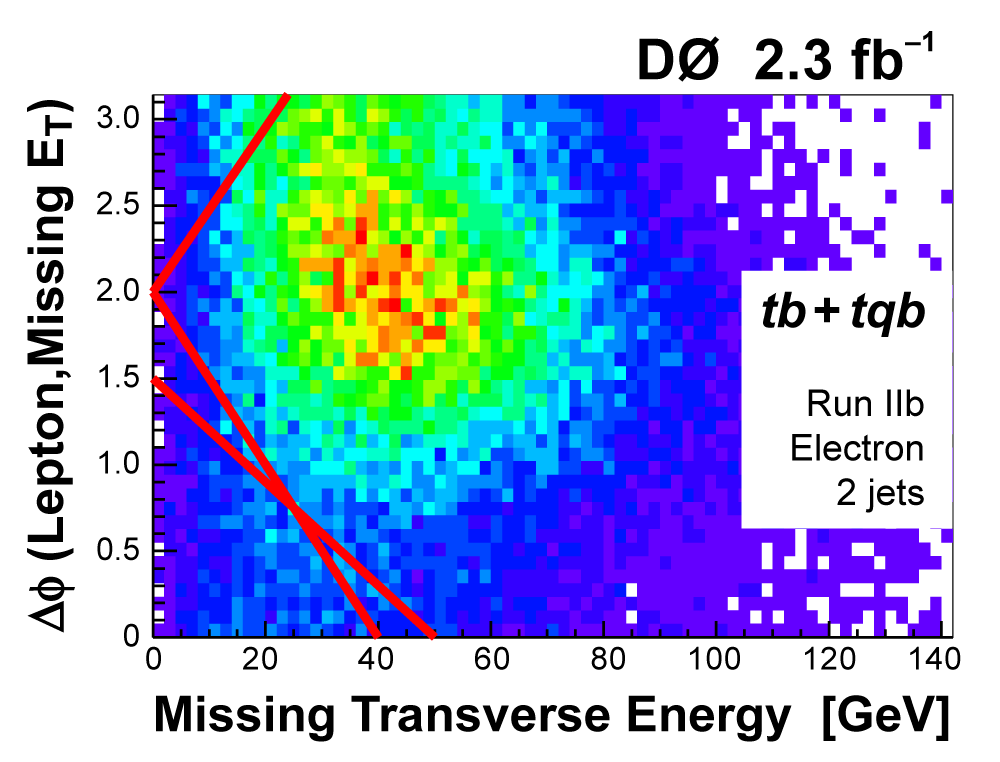
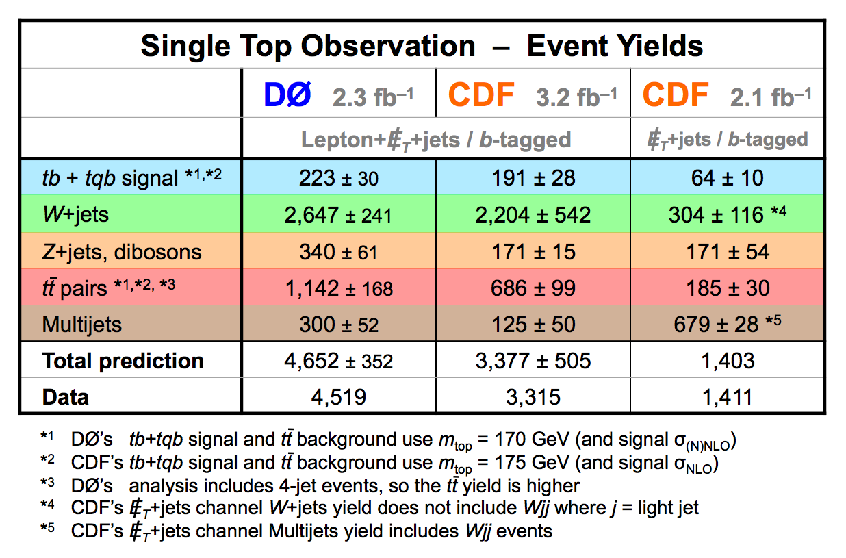
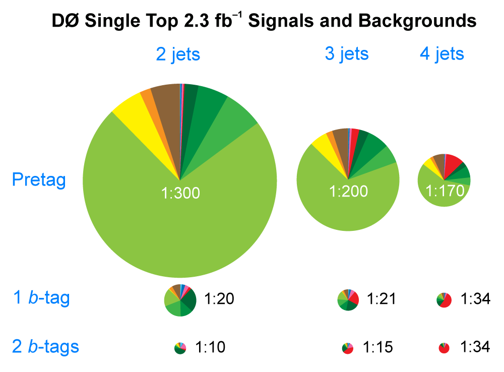
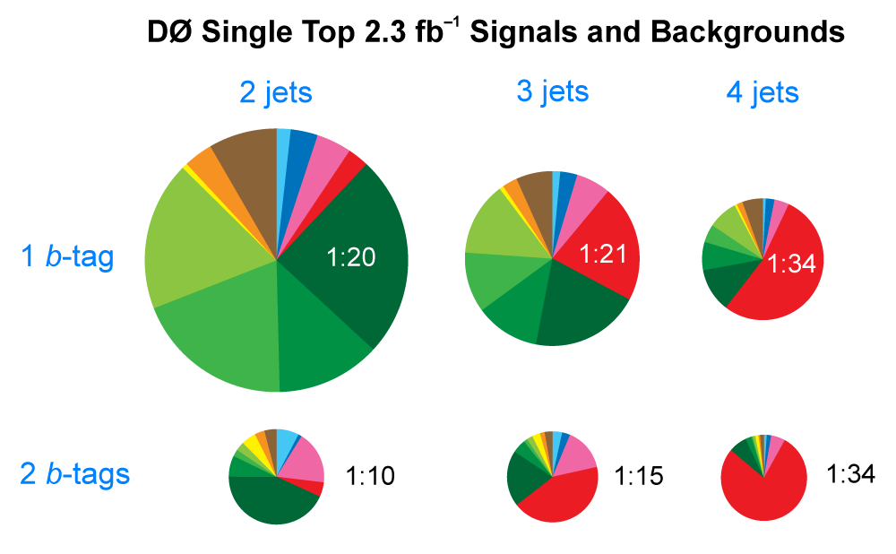
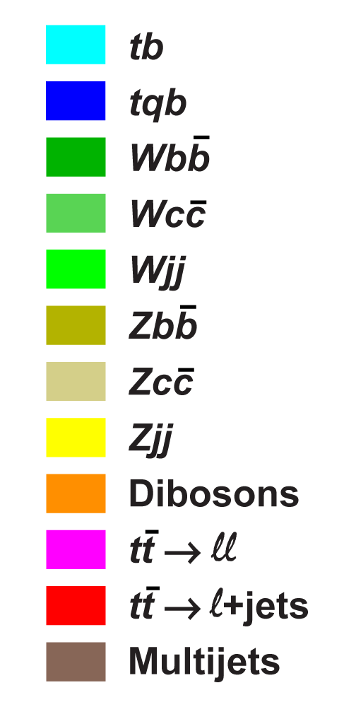
The measurement uses data that pass almost any online trigger for maximum efficiency. We require between two and four jets, exactly one high transverse momentum electron or muon isolated from all jets in the event, and high missing transverse energy. One or two of the jets must be b-tagged. We model the single-top signal using the COMPHEP-SINGLETOP event generator coupled to PYTHIA for the underlying event and jet fragmentation. We model the tt, W+jets, and Z+jets using ALPGEN with PYTHIA using parton-jet matching. The small diboson (WW, WZ, ZZ) backgrounds are modeled with PYTHIA and the small multijet backgrounds where a jet has faked an electron, or a muon from b decay has traveled wide of its jet, is modeled using data. The tt, Z+jets, and diboson backgrounds are normalized to the theory cross sections, and the W+jets and multijets backgrounds are normalized to data. The resulting event yields are shown in the tables below. The proportions of signal and background predicted in the data before and after b-tagging are shown in the pie charts. After event selection, the signal acceptances (percentage of total cross section that pass the cuts) are (3.7 ± 0.5)% for the s-channel tb process and (2.5 ± 0.3)% for the t-channel tqb process. (The t-channel process has a lower acceptance because the second b-jet has low transverse momentum and is difficult to identify. These acceptances are ~18% higher than in our previous analysis, mainly because of the change in choice of triggers from lepton+jets ones only to allowing data events to pass almost any trigger. This analysis uses 85 million Monte Carlo events. After event selection, we have 0.5 million MC signal events, 1.4 million W+jets events, 1.6 million tt, a few hundred thousand Z+jets and diboson events, (4.1 million MC events in total), and 0.8 million pretagged multijets data events (31 thousand with b-tags).

Yields Before b-Tagging

Pretag event yields in the 2.3ifb analysis

B-Jet Identification

We use a neural network b-tagging algorithm with two cut-points. The "tight" b-tagging ID used for single-tagged events has an efficiency of 40% for identifying b-jets, with a 9% probability to tag c-jets and 0.4% for light-quark jets. The "loose" b-tagging ID used for double-tagged events has an efficiency of 50% for identifying b-jets, with a 14% probability to tag c-jets and 1.5% for light-quark jets. (These efficiencies include the losses from the incomplete geometric acceptance of the Silicon Microstrip Tracker. For jets within the SMT acceptance, the efficiencies are 47% b's), 10% (c's), and 0.5% (light-jets) for tight tagging, and 58% (b's), 17% (c's), and 1.8% (light-jets) for loose tagging.) To model the b-tagging in Monte Carlo events we parametrize the efficiency in "tag-rate functions" as a function of jet transverse momentum and jet pseudorapidity separately for each jet flavor, and then apply these probabilities to every combination of jets in every MC event (using "the permuter") to obtain a tag probability for each event. Before b-tagging, the signal:background ratios vary from 1:300 in the 2-jets channel to 1:170 in the 4-jets channel (average 1:260). After b-tagging, this is improved to values ranging from 1:10 to 1:37, depending on the analysis channel, with the most powerful channel (2jets/1-tag) and the average of all channels having S:B = 1:20.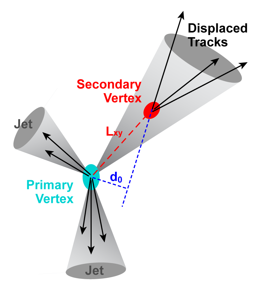

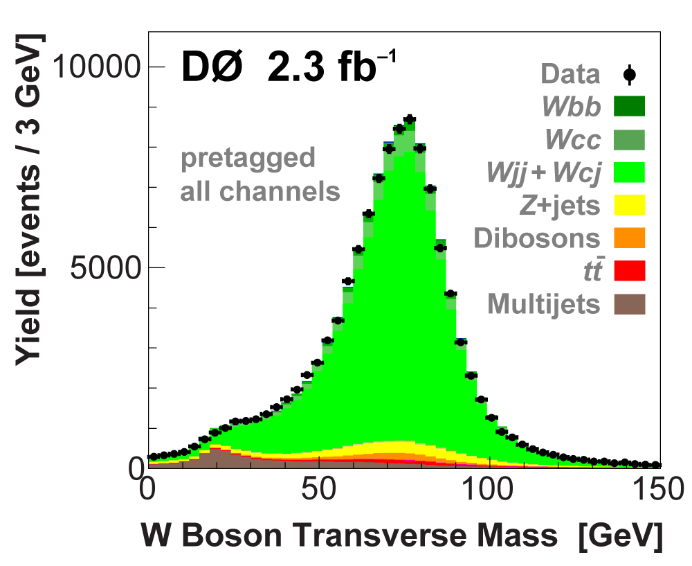
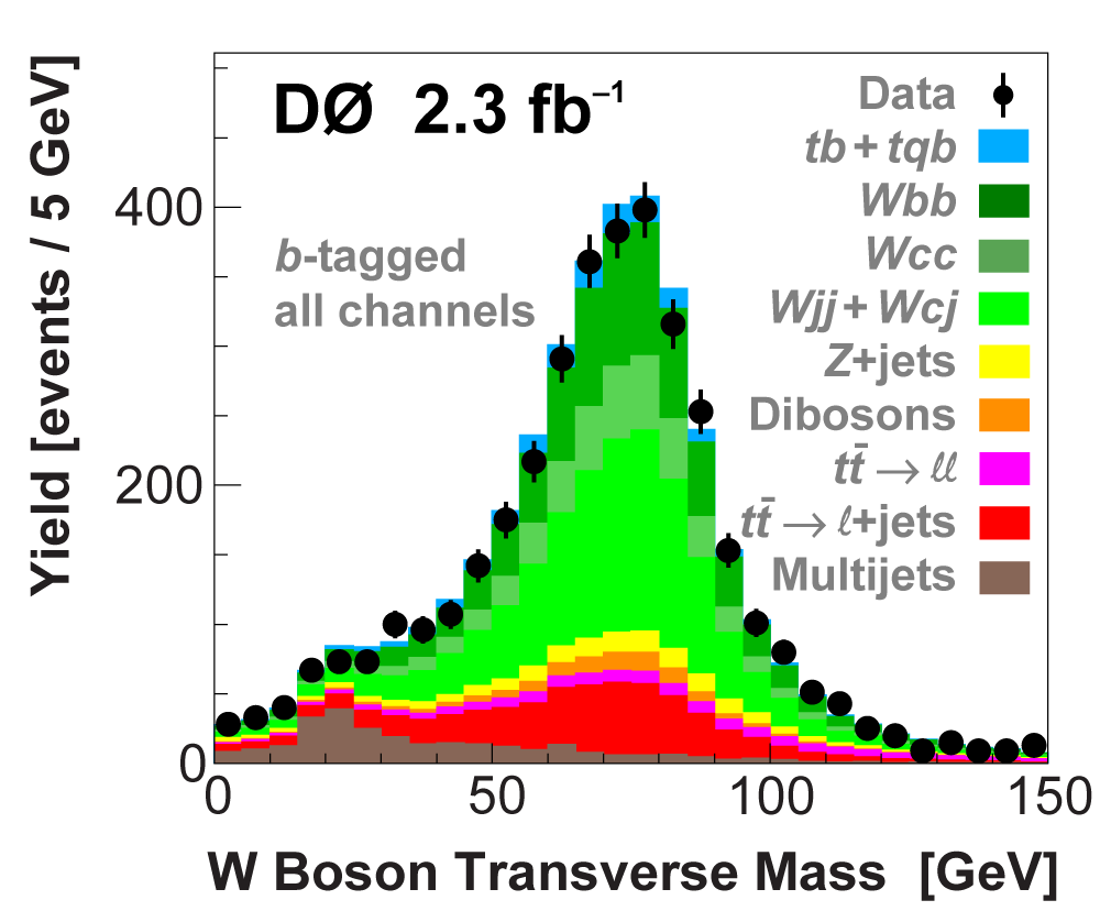
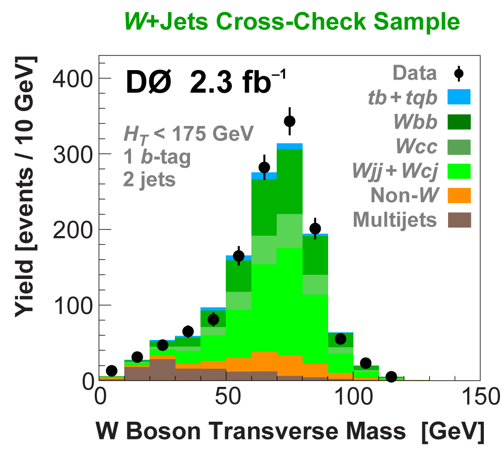
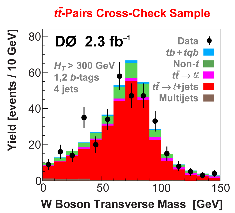
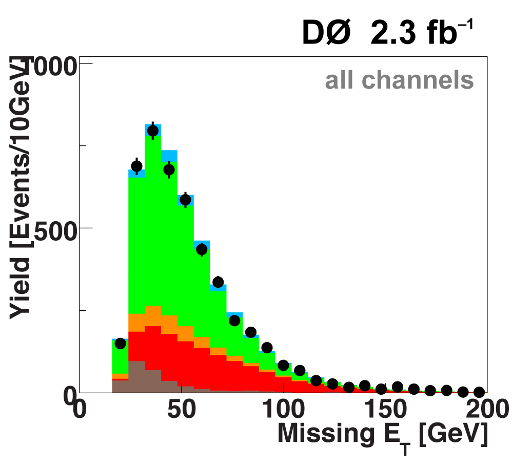
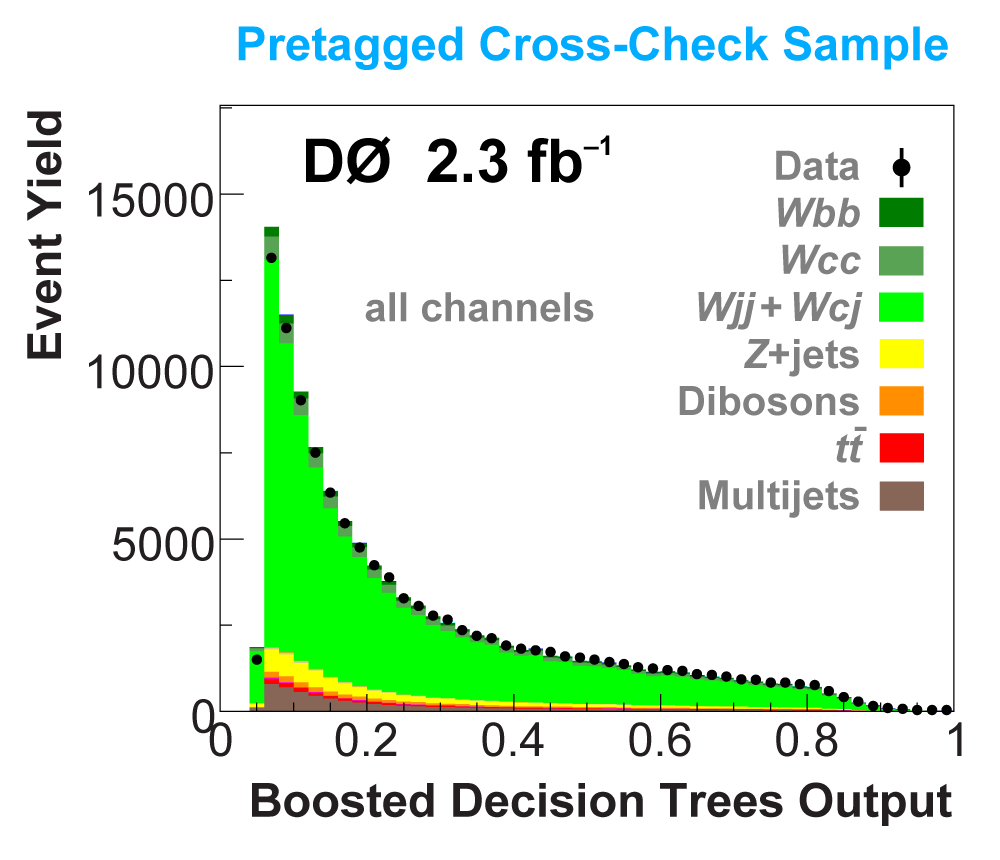
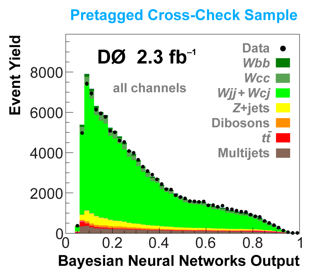
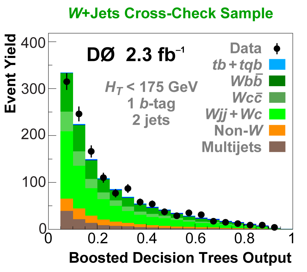
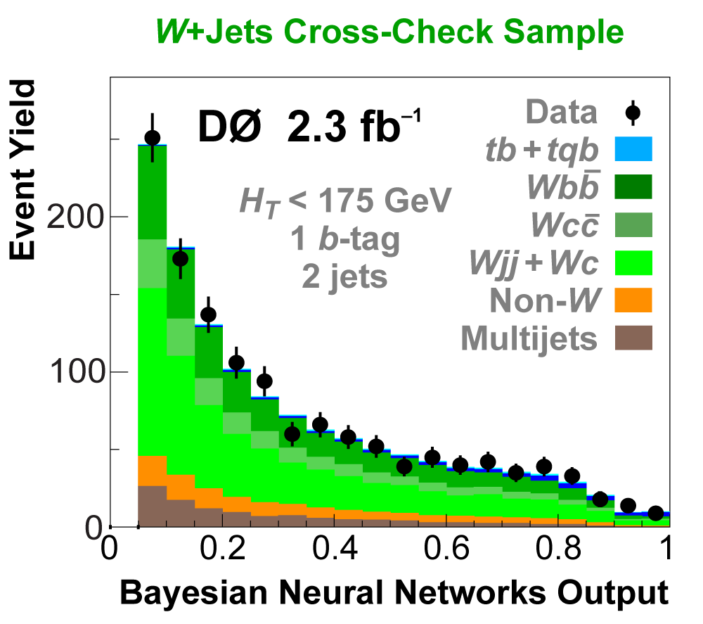
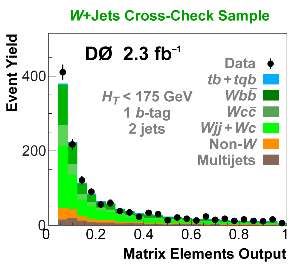
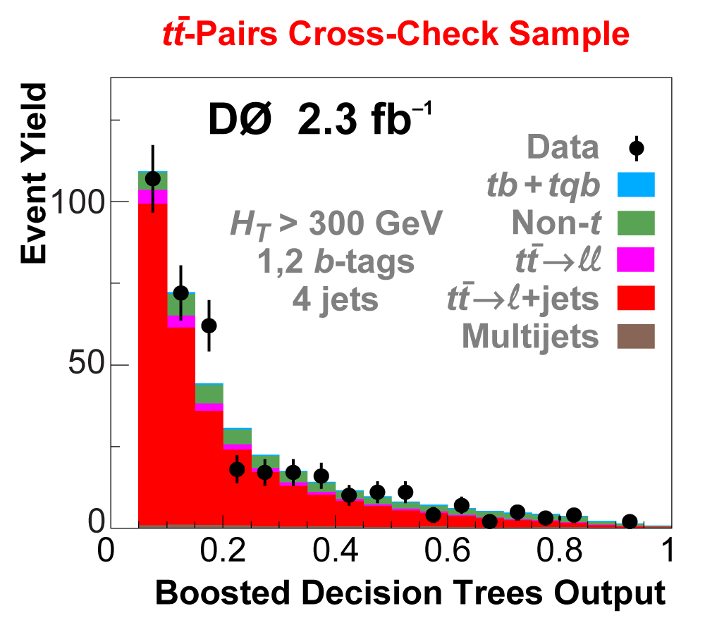
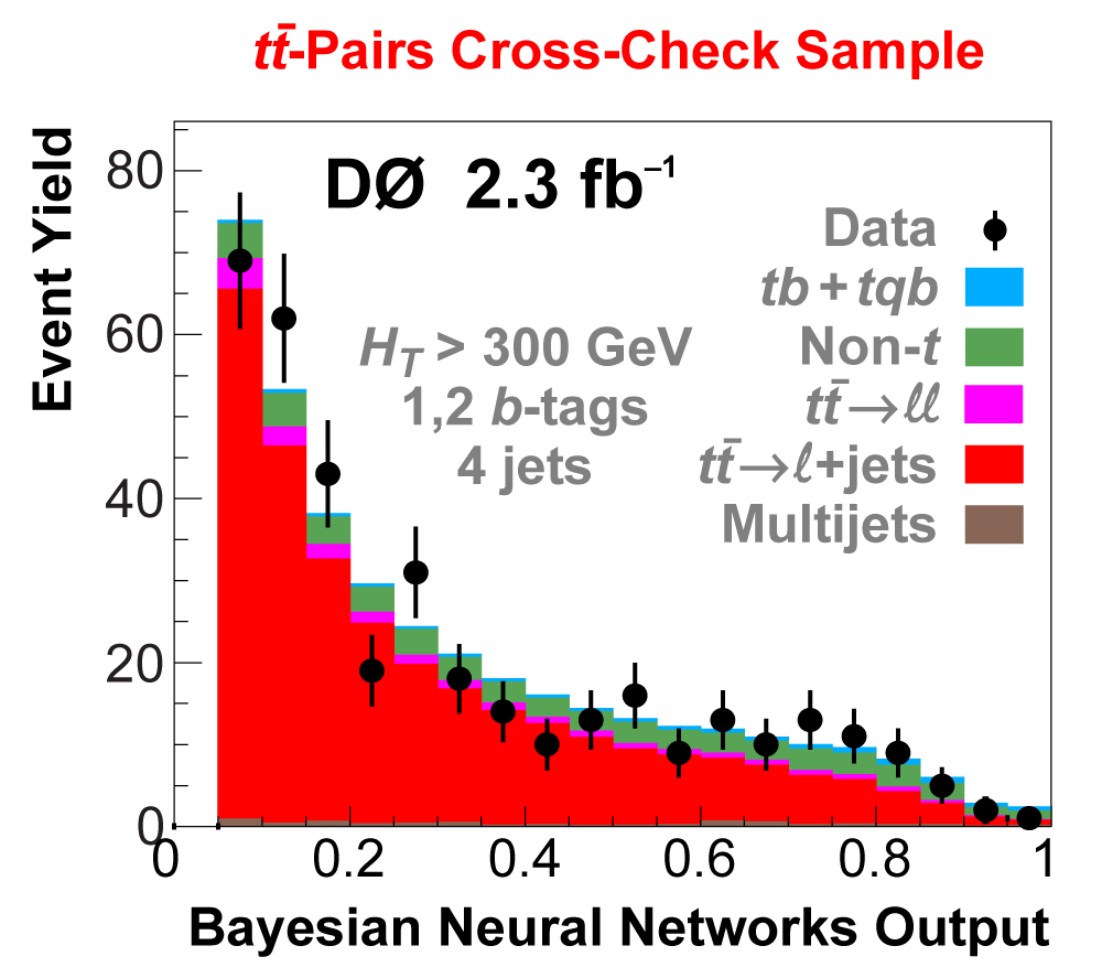
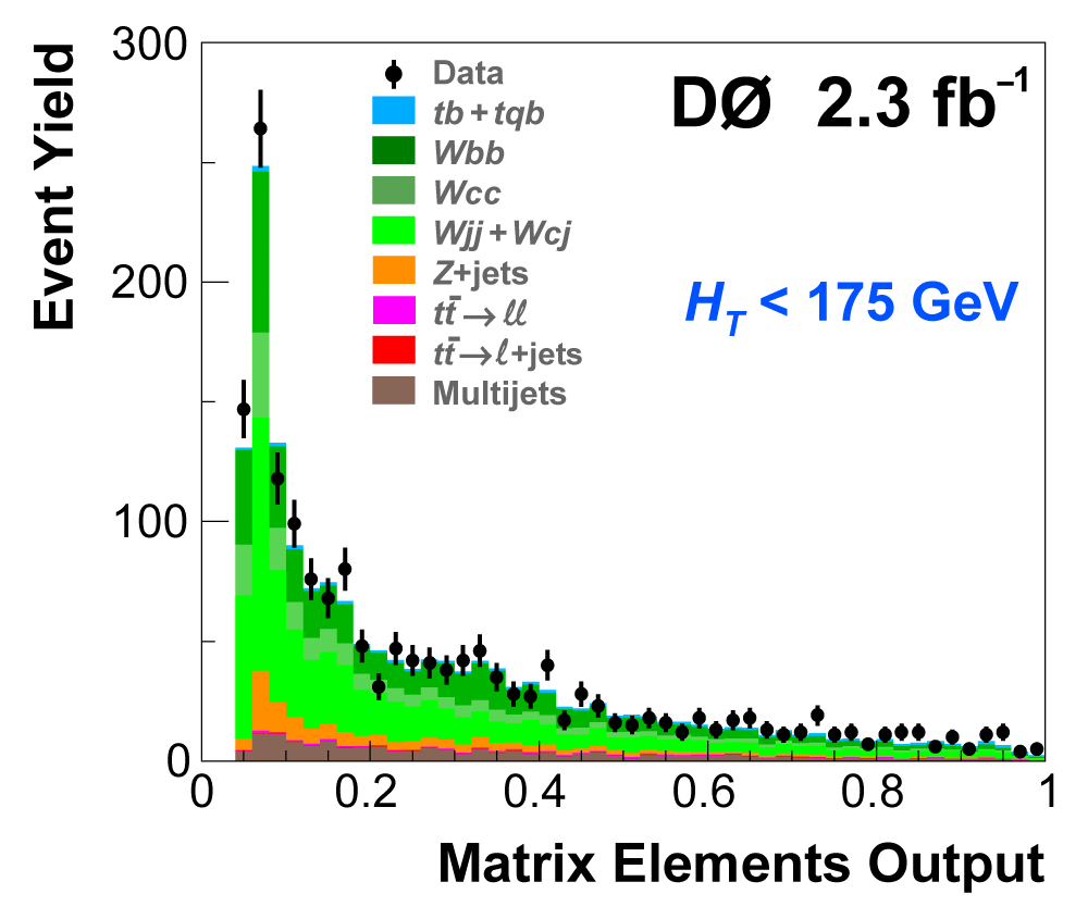
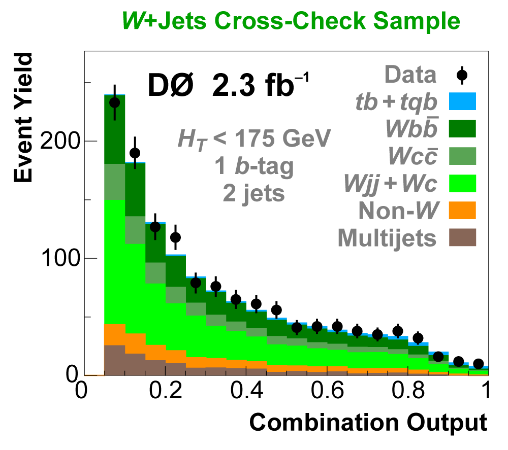
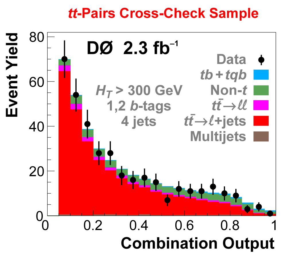
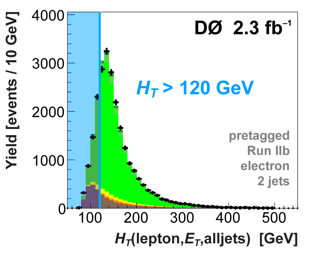
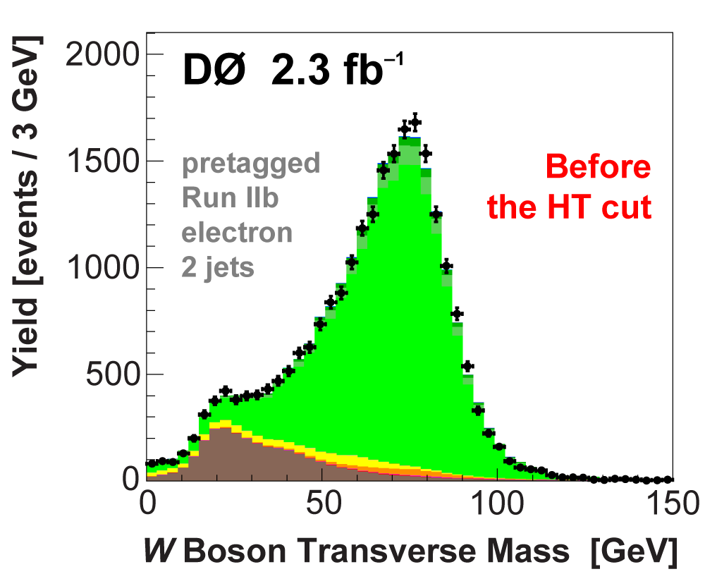
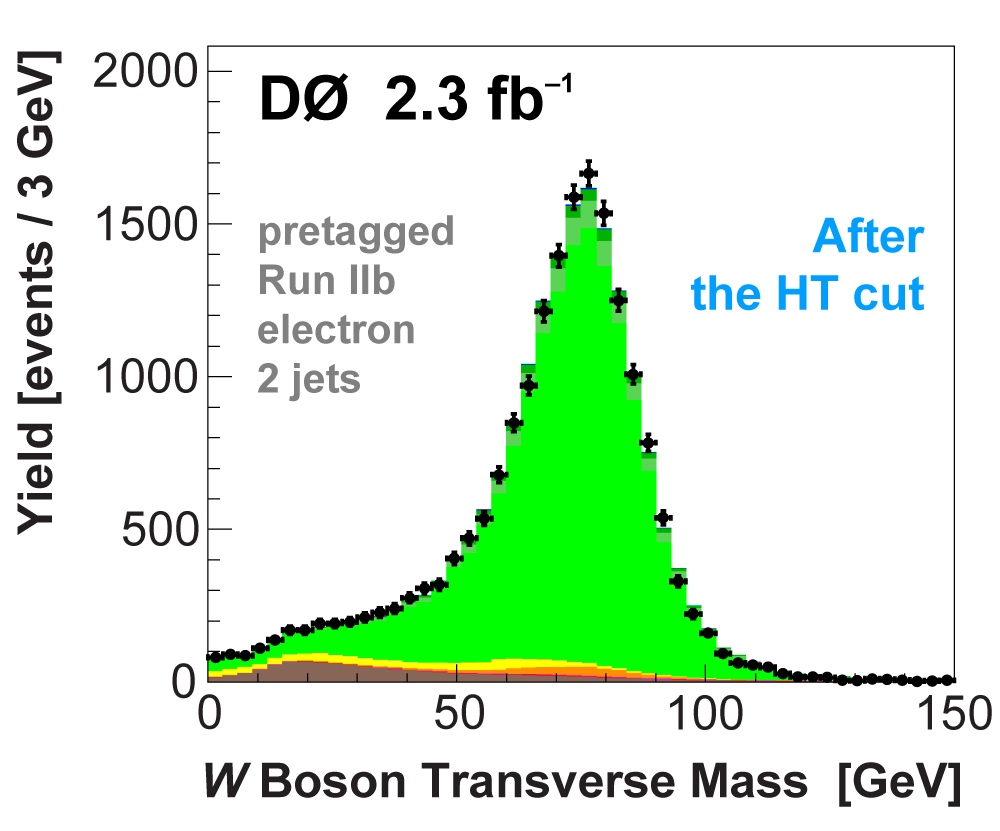
Yields After b-Tagging

Tagged event yields in the 2.3ifb analysis

More Detailed Yield Information

Background pie charts, separate channels

Cross Checks

We perform the analysis in 24 independent analysis channels (Run IIa, Run IIb; electron, muon; 2,3,4 jets; 1,2 b-tags) to take advantage of the different signal:background ratios and dominant sources of background. In additional to checking the distributions of about 160 variables for data-background agreement in all analysis channels separately, before and after b-tagging , we also define two cross-check samples to check the background model components separately. The first sample has low total energy (exactly two jets and the total transverse energy H_T(lepton,neutrino,alljets) < 175 GeV), and only one b-tagged jet, to maximize the W+jets content and minimize the top pairs contribution, and the second sample has high total energy (exactly four jets and H_T > 300 GeV), and one or two b-tagged jets, to maximize the top pairs component and minimize the W+jets contribution. We find good agreement for both normalization and shape in all variables studied. The W boson transverse mass distribution is shown here as an example.

Systematic Uncertainties

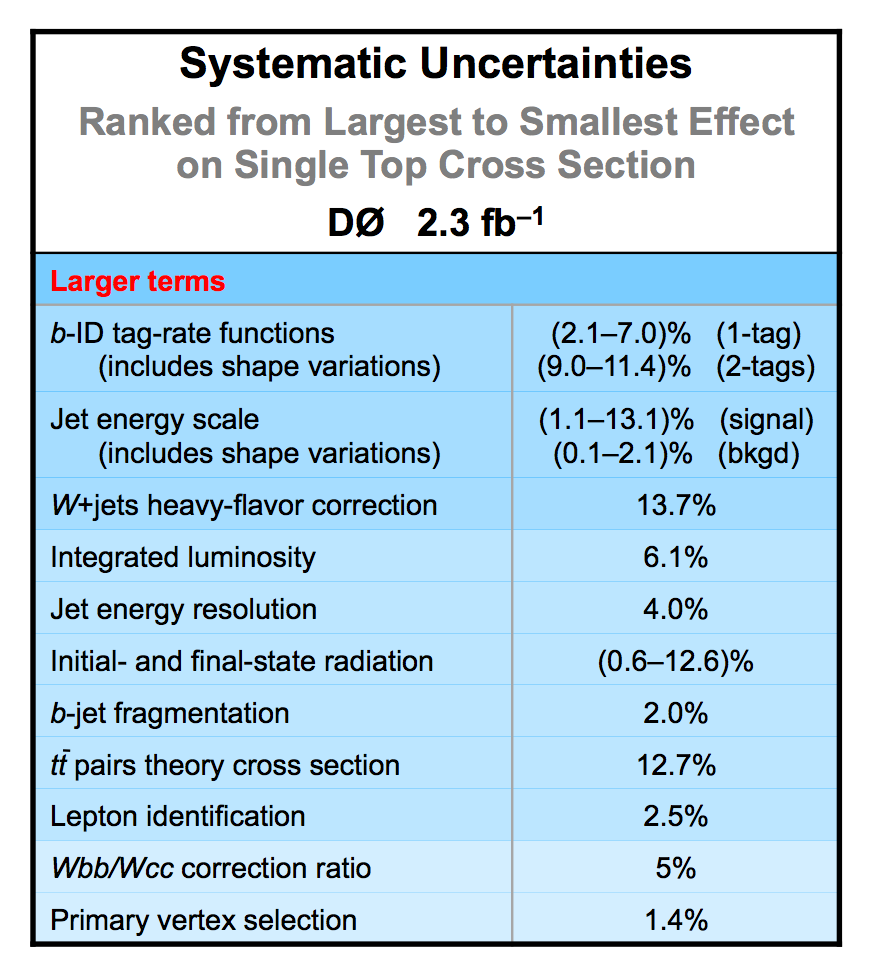
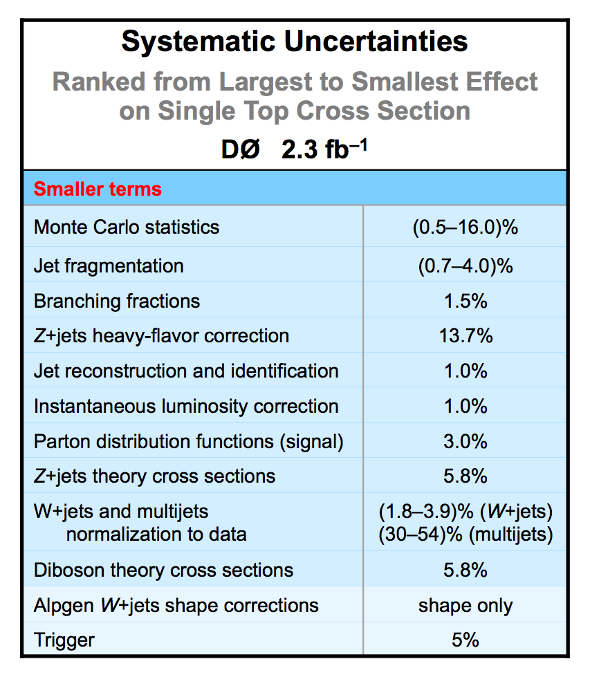
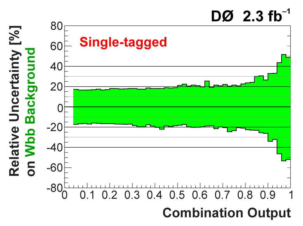
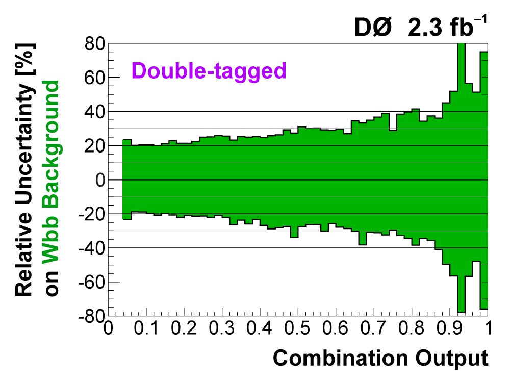
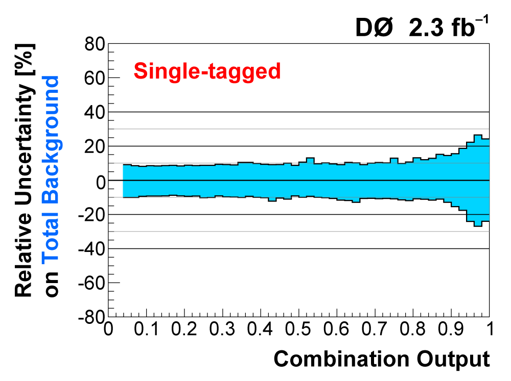
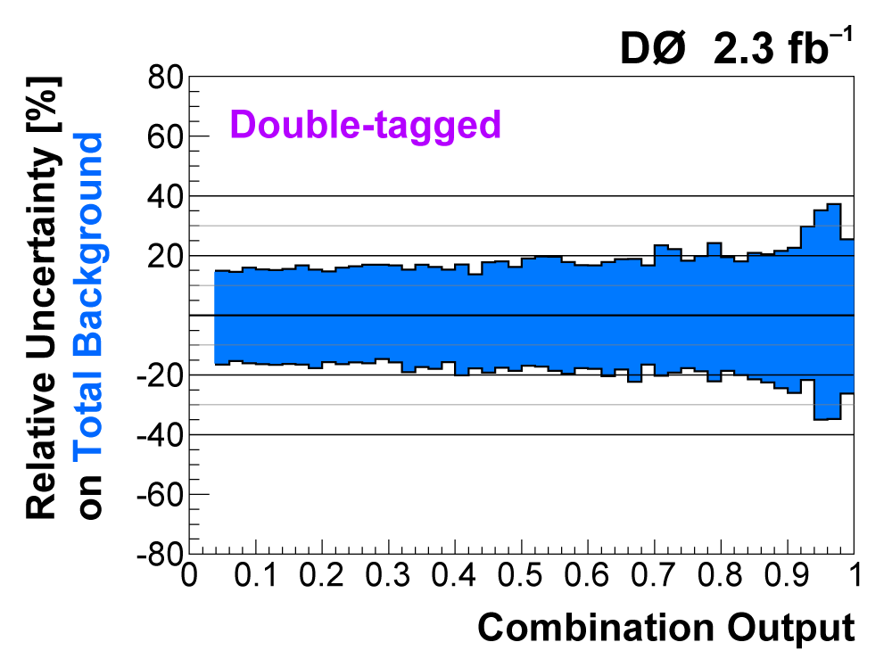
The uncertainties in all searches are dominated by the statistical uncertainty from the size of the data sample. However, once there is enough data to observe and measure something, then systematic contributions to the total uncertainty become important. The total uncertainty on the single top cross section measured in this observation analysis is ±22%. When we perform the calculation without including any systematics, it is 18% (i.e., this is the statistical uncertainty). Thus, the systematic component of the total cross section is approximately 13%. We consider both normalization systematic uncertainties and shape-dependent systematic uncertainties separately for each signal and background source in each analysis channel. The overall background uncertainty varies between 7% and 15% for the individual channels. Shape uncertainties result in 20% to 40% uncertainties in the discriminant output region near one. The following two tables show the sources of systematic uncertainty included in this measurement, in ranked order of contribution to the total cross section uncertainty. Other potential sources of systematic uncertainty were studied and found to have a negligible effect.

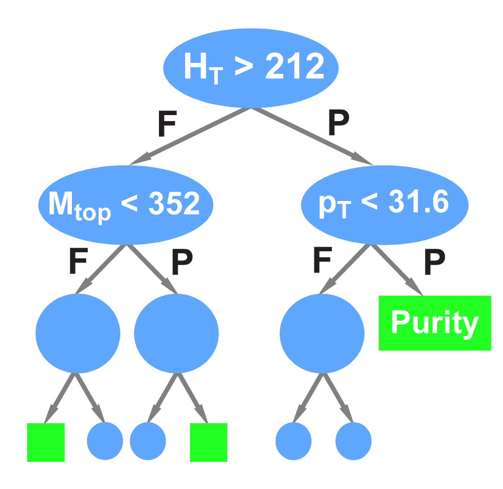
Systematic uncertainties in the single top analysis, smaller ones

Signal-Background Discrimination

We apply three methods to separate signal from background:

Boosted Decision Trees. A decision tree applies sequential cuts to the events but does not reject events that fail the cuts. Boosting averages the results over many trees and improves the performance by about 20%. We use 50 boosting cycles. The most important part of a boosted decision tree analysis is the choice of variables. We use the highest ranked (most discriminating) 64 variables from the 97 shown below (chosen to have good agreement between data and background in all analysis channels as well as having different distributions for signal and at least one background component). We use the same variables in all analysis channels.
Bayesian Neural Networks. A neural network is trained on signal and background samples to obtain weights between the network nodes and thresholds at the nodes. Bayesian neural networks average over a large number of such networks to improve the performance. We average over 100 networks. The most important part of a Bayesian neural network analysis is the choice of variables. We use the highest ranked 18–28 variables from the ones shown below, with a different set optimized for each analysis channel. The networks each have 20 hidden nodes.
Matrix elements. This method was pioneered by DØ in the top quark mass measurement. It uses the 4-vectors of the reconstructed lepton and jets (inlcuding the jet flavor information) and the Feynman diagrams for 2-jet and 3-jet events to compute an event probability density for the signal and background hypotheses. We use the matrix elements for 19 Feynman diagrams for signal and backgrounds (×2 for charge conjugate states) to separate them. To improve the performance, we split the data into events with low total transverse energy (that have mainly W+jets in the background) and events with high total transverse energy (that have most of the top pair background events).

Cartoons of the BDT and BNN Techniques and an Example of BNN Averaging

The Matrix Elements

Discriminating Variables

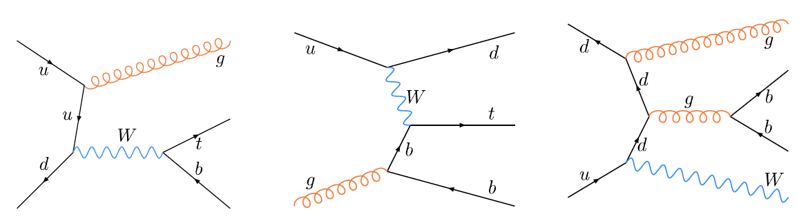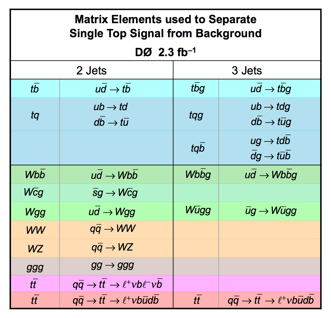
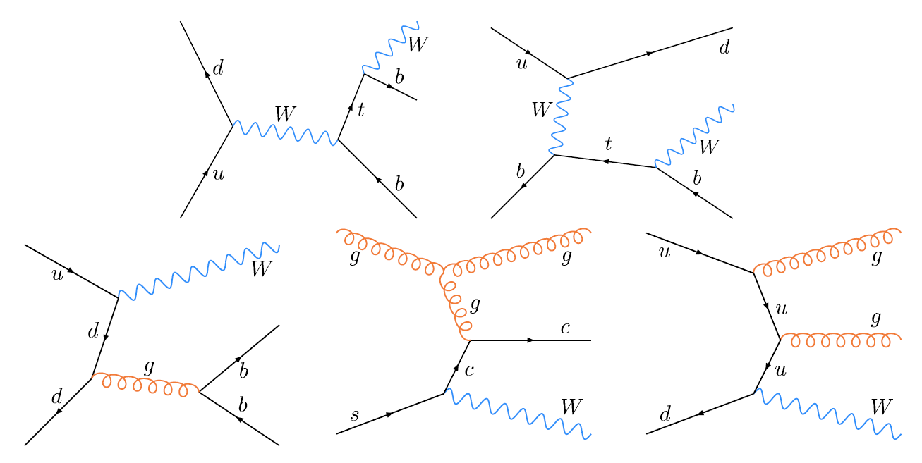
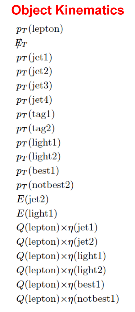
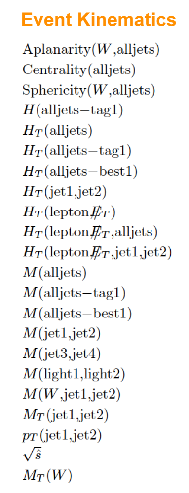
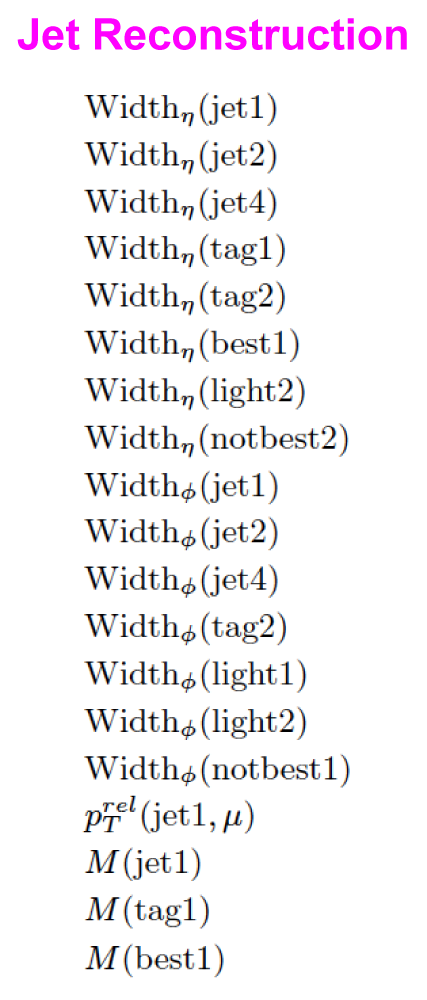
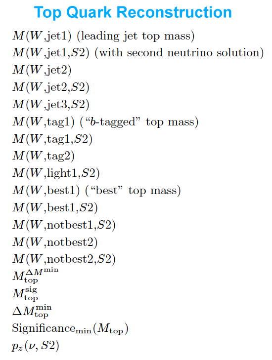
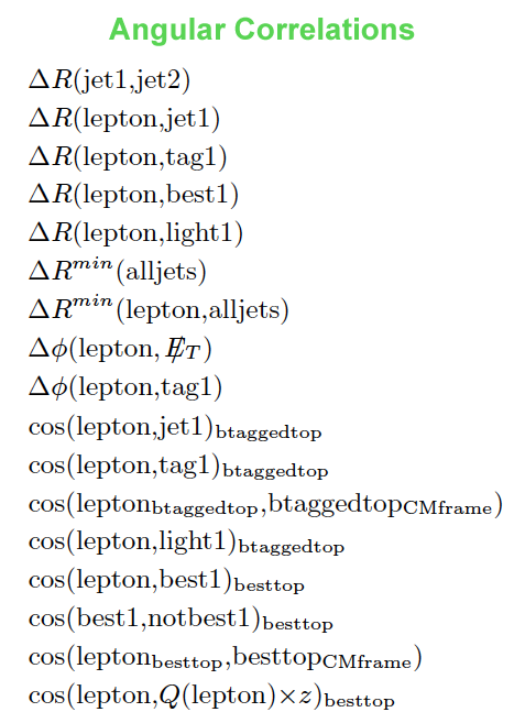
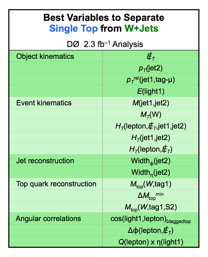
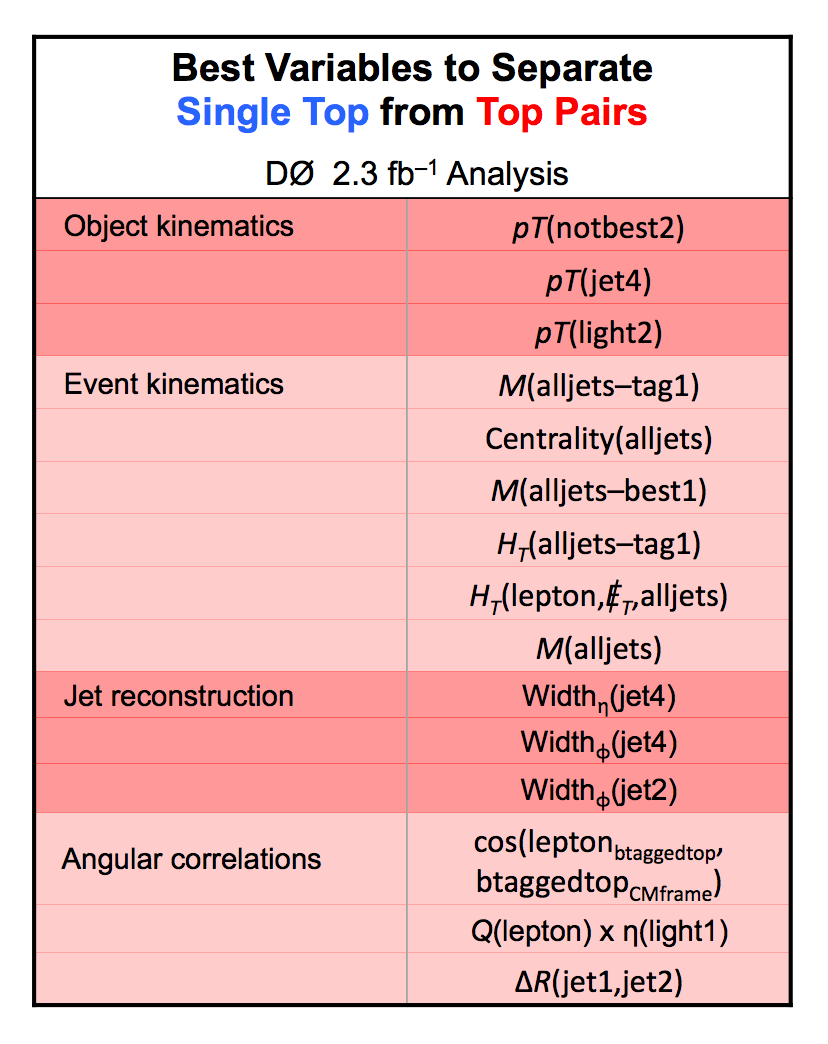
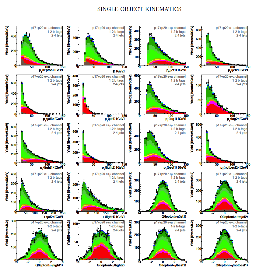
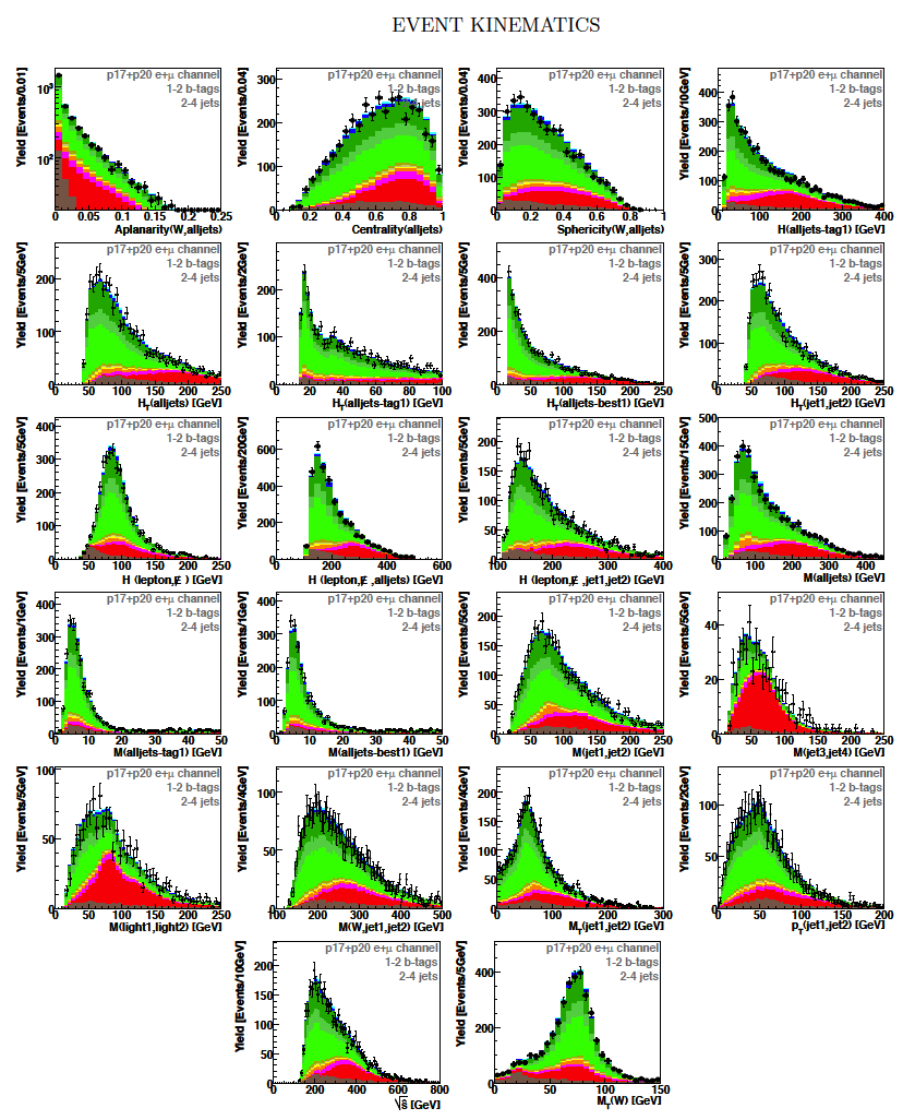
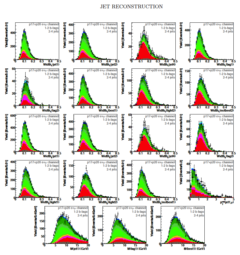
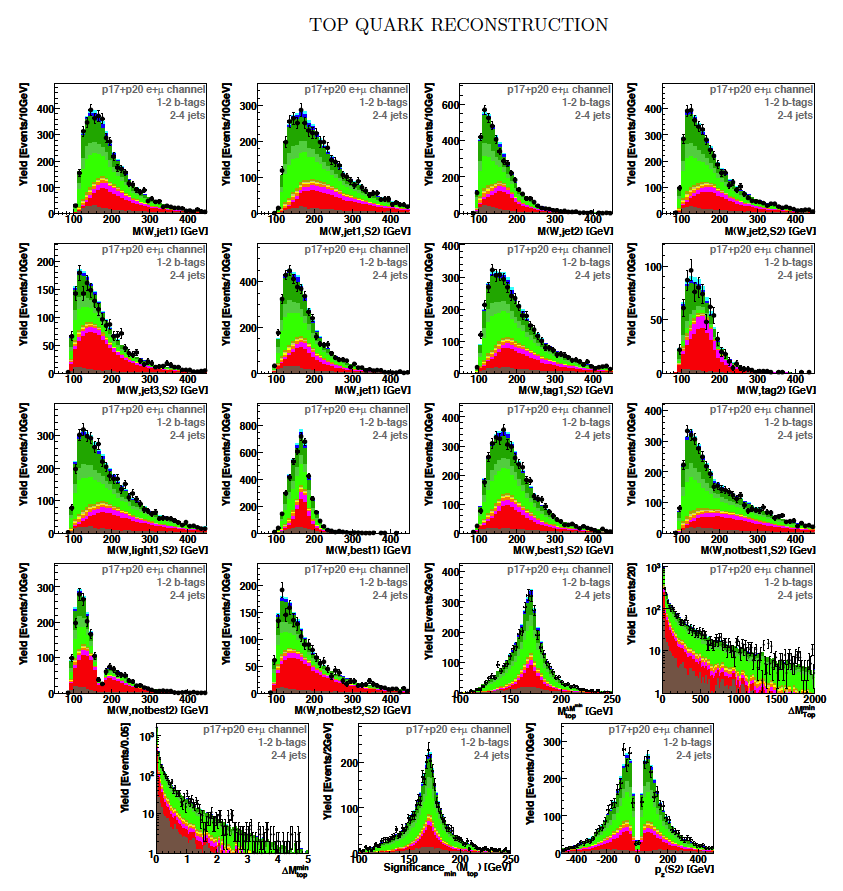
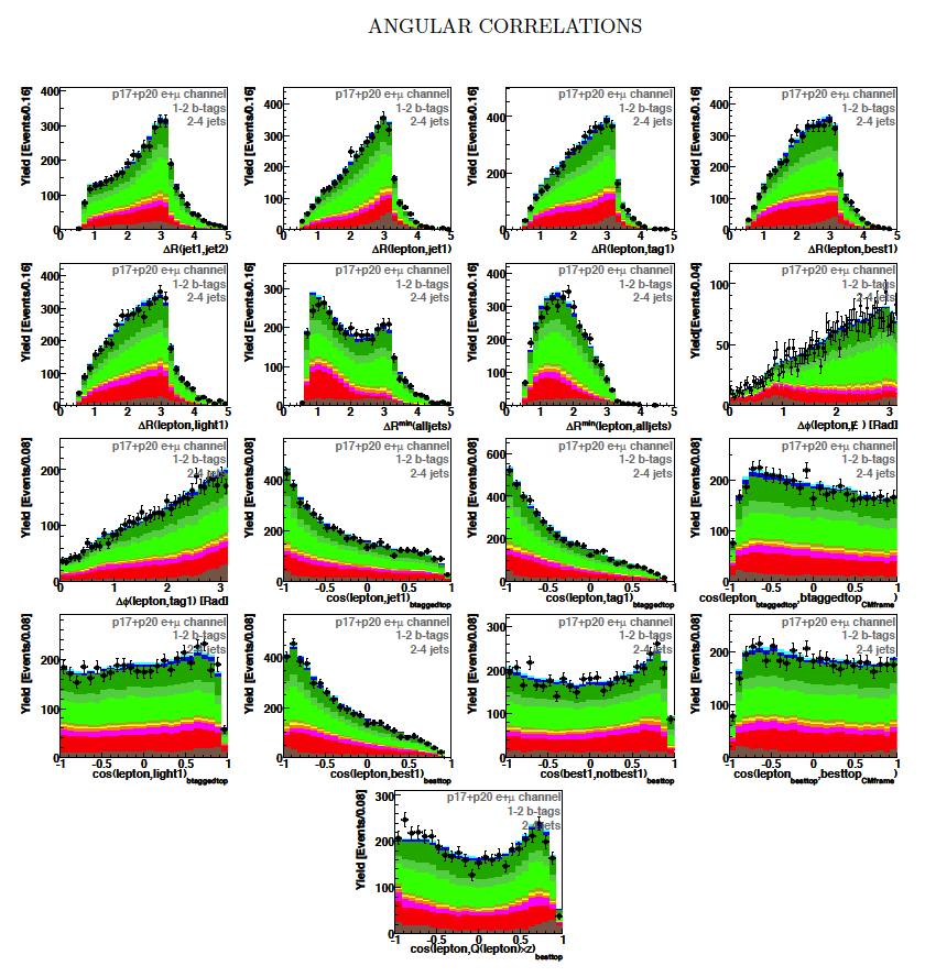
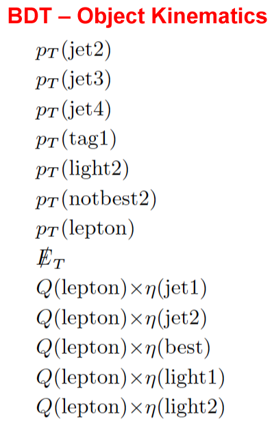
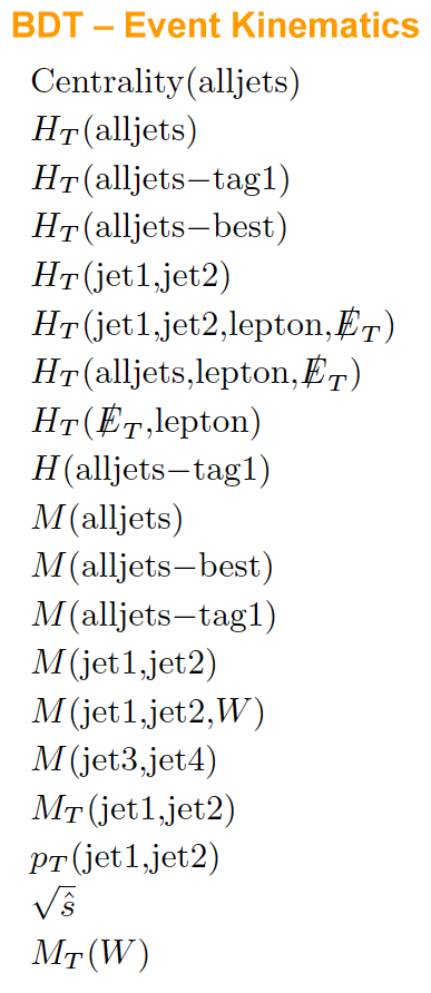
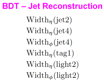
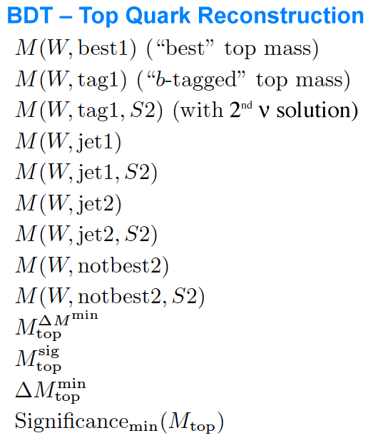
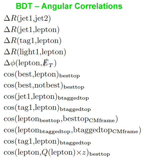
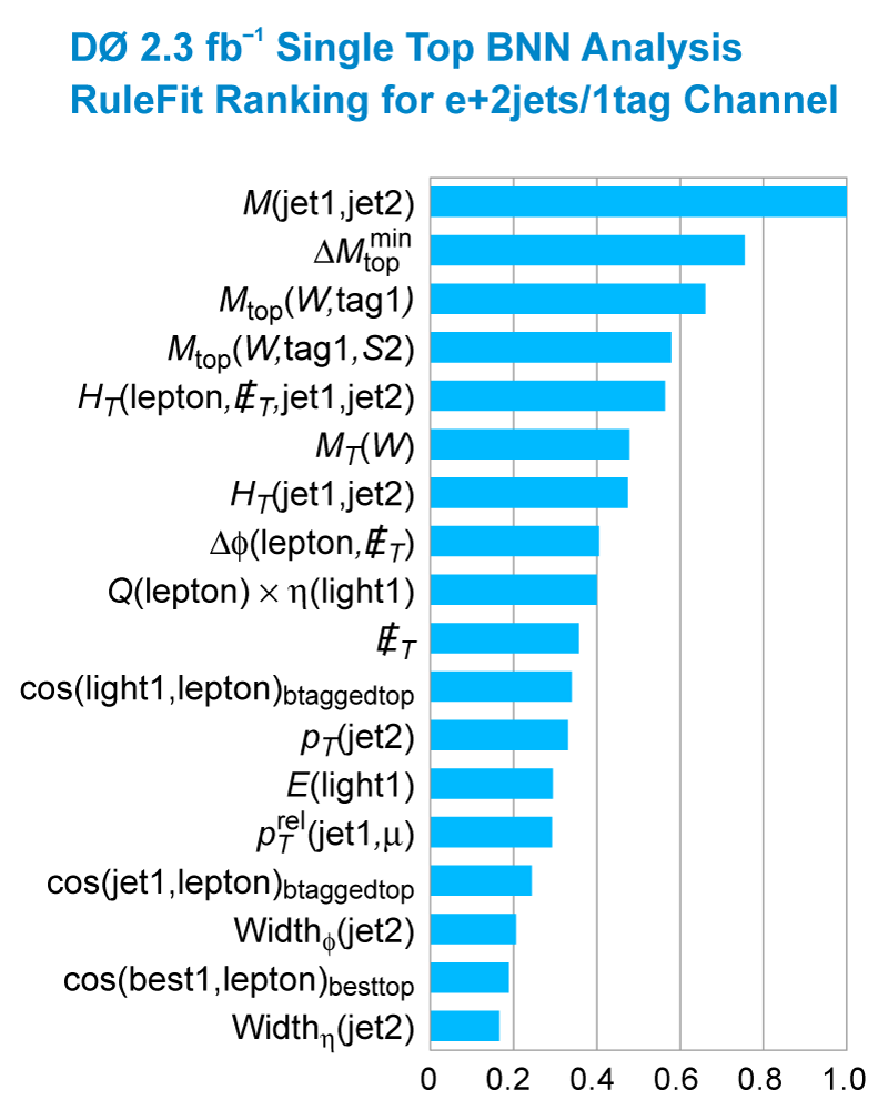
These tables show the variables used by the boosted decision trees and the Bayesian neural networks. (Plots of all variables are at the bottom of the page.) Some comments on the notation are in order. The numbering n of jetn, tagn, lightn, etc. refers to the transverse momentum ordering of the jets, 1 is the highest p_T jet of that type of jet, 2 is the second-highest p_T jet, and so on. "tag" means a b-tagged jet. "light" means an untagged jet (it failed the b-tag criteria). "best" means the jet which, when combined with the lepton and missing transverse energy, produces a reconstructed top quark mass closest to 170 GeV (the value at which we did the analysis). "notbest" means any jet that is not the best jet. "alljets" means include all the jets in the event in the global variable (there are 2, 3, or 4 of them). p_T is the transverse momentum. E is the particle energy. Q is the particle's charge. H is the scalar sum of the particles' energies. H_T is the scalar sum of the transverse energies. M is the invariant mass of the objects. M_T is the transverse mass of the objects. Sqrt(s^hat) is the total center of mass energy in the event. p_T^rel is the transverse momentum of the muon relative to the closest jet. S1 and S2 are the two solutions for the neutrino longitudinal momentum when solving the W boson mass equation, and S1 is the smallest absolute value of the two (the preferred value). M_top^ΔMmin is the reconstructed top quark mass using the jet and neutrino solution that make the mass closest to 170 GeV. ΔM_top^min is the difference in GeV between M_top^ΔMmin and 170 GeV. M_top^sig is the reconstructed top quark mass using the jet and neutrino solution that gives the lowest value for "significance," where Significance_min(M_top) is log_e of the jet and missing transverse energy resolution functions calculated at M_top divided by the resolution functions at 170 GeV. ΔR is sqrt(Δφ² + Δη²).

Which Variables are Most Powerful?

Best variables to separate single top from W+jets

Best variables to separate single top from ttbar

Example Variable Distributions for Each Variable Category

Discriminant Output Transformation

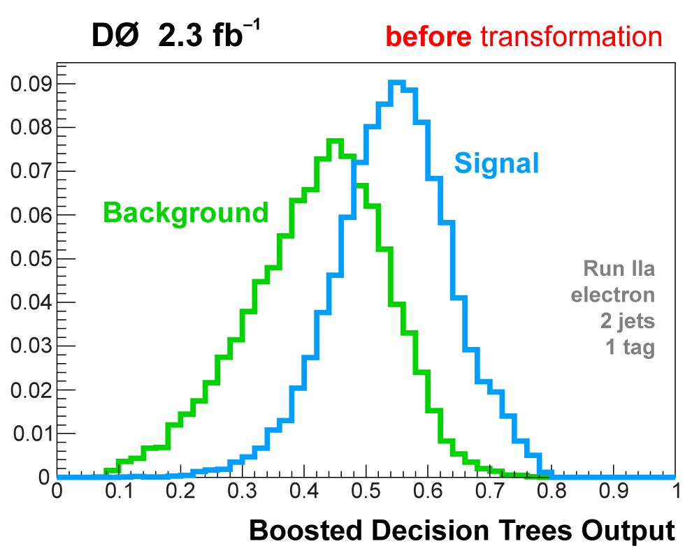
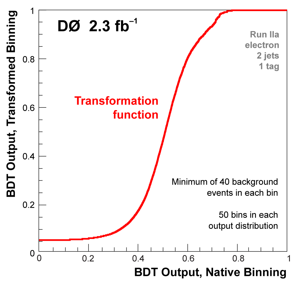
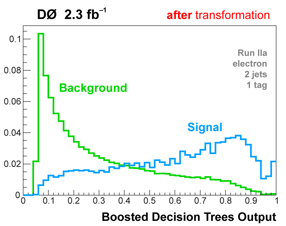
All raw discriminant output distributions undergo a monotonic transformation of the binning to ensure that every bin (50 in each distribution) has at least 40 background events, so that there are no bins with a nonzero signal prediction or data but not enough background in the model to use that information. The bins from the matrix elements outputs are then also reordered in descending signal:background ratio from 1 towards 0. After transformation, analysis channels with lower statistics do not have entries in all 50 bins, the filled bins start at one and end before reaching zero. The following plots illustrate the output transformation process for one channel in the boosted decision trees analysis.

Decision tree output before transformation

Decision tree output after transformation

Discriminant Performance

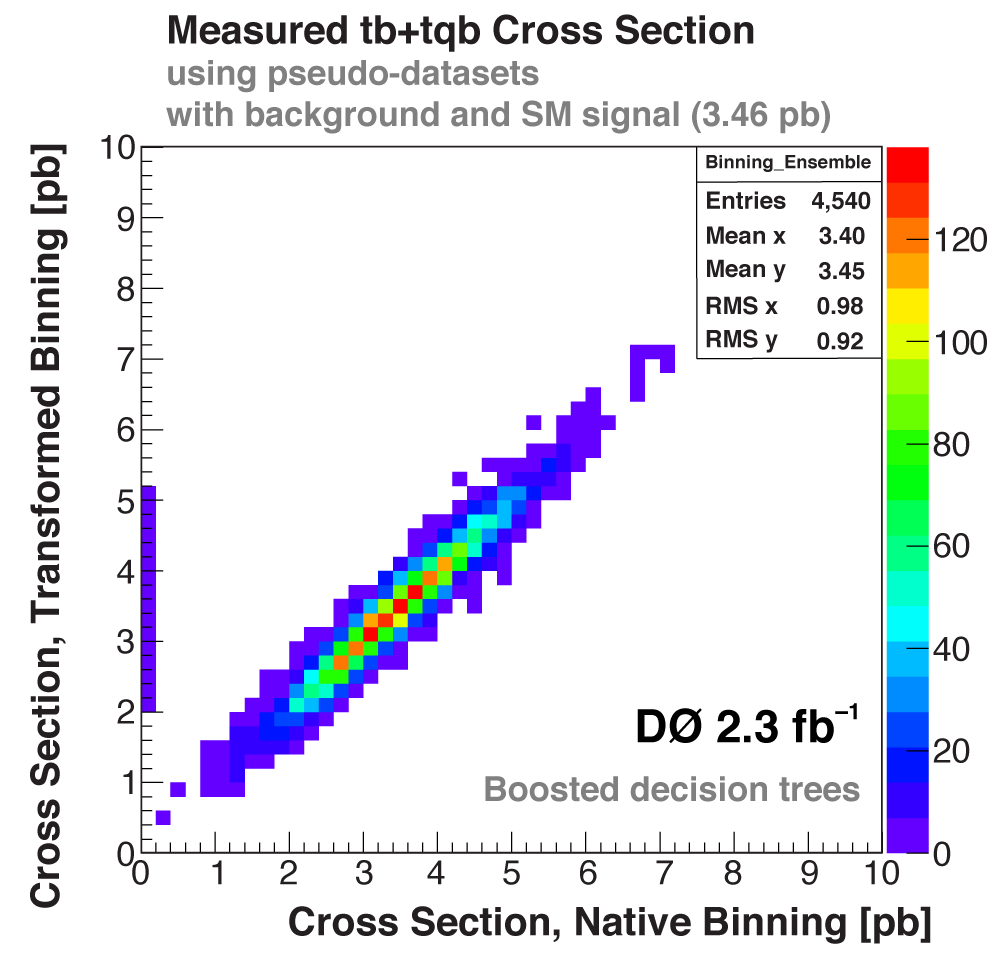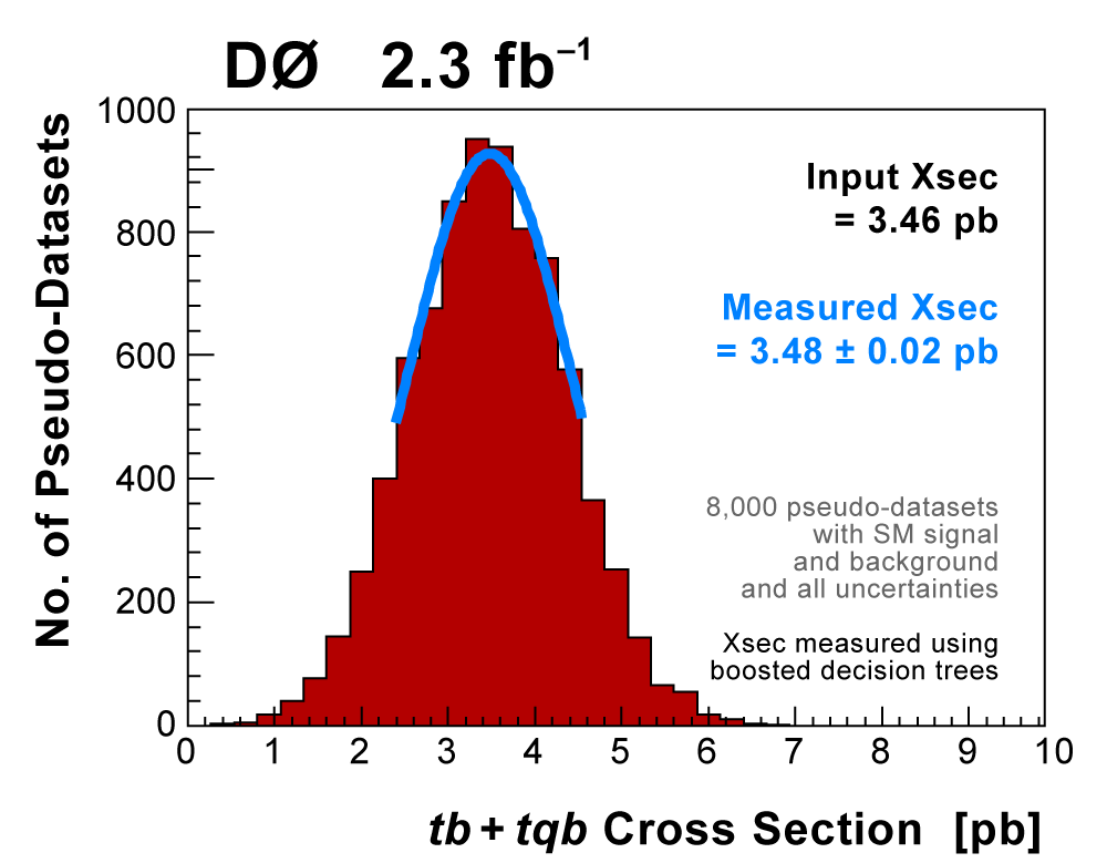
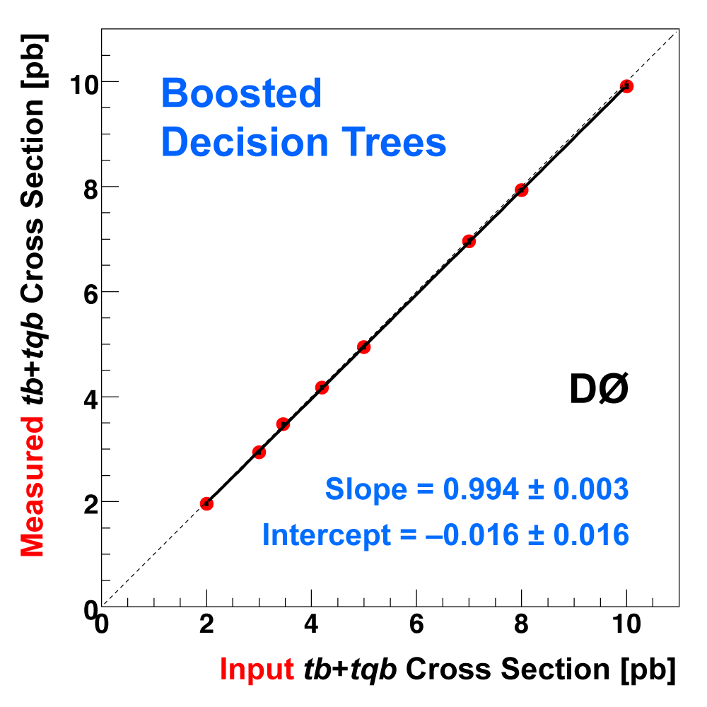
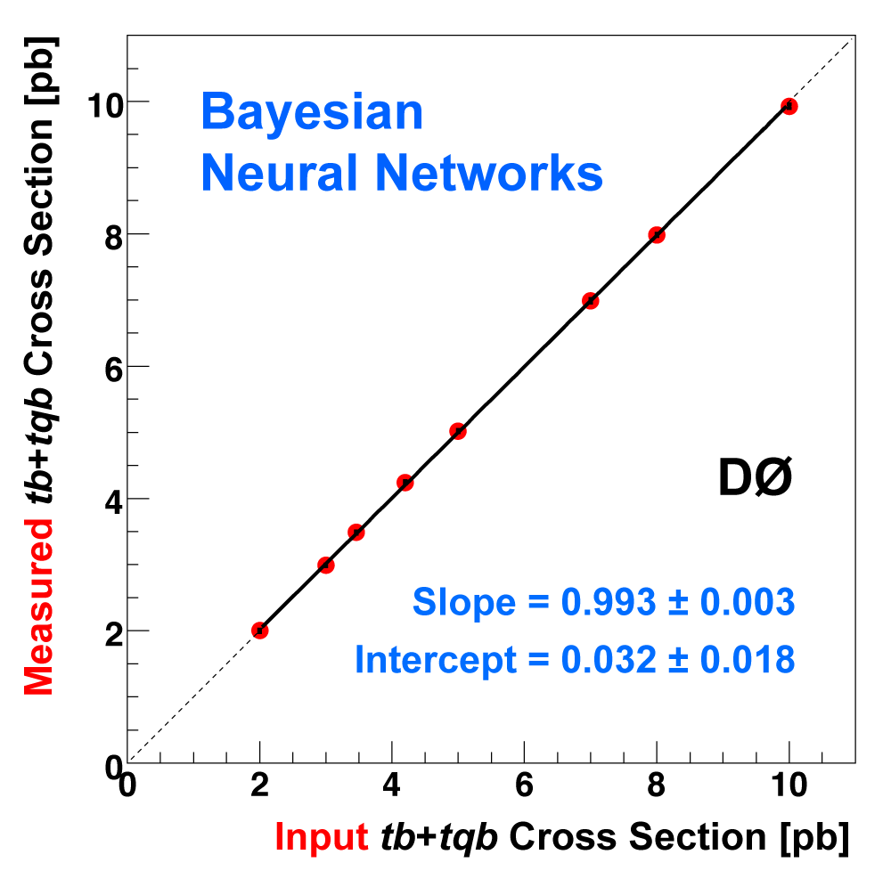
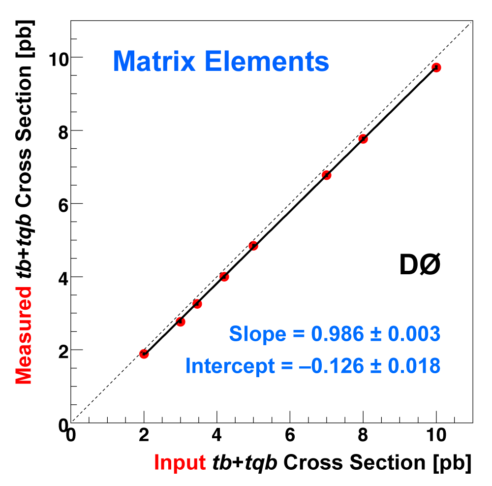
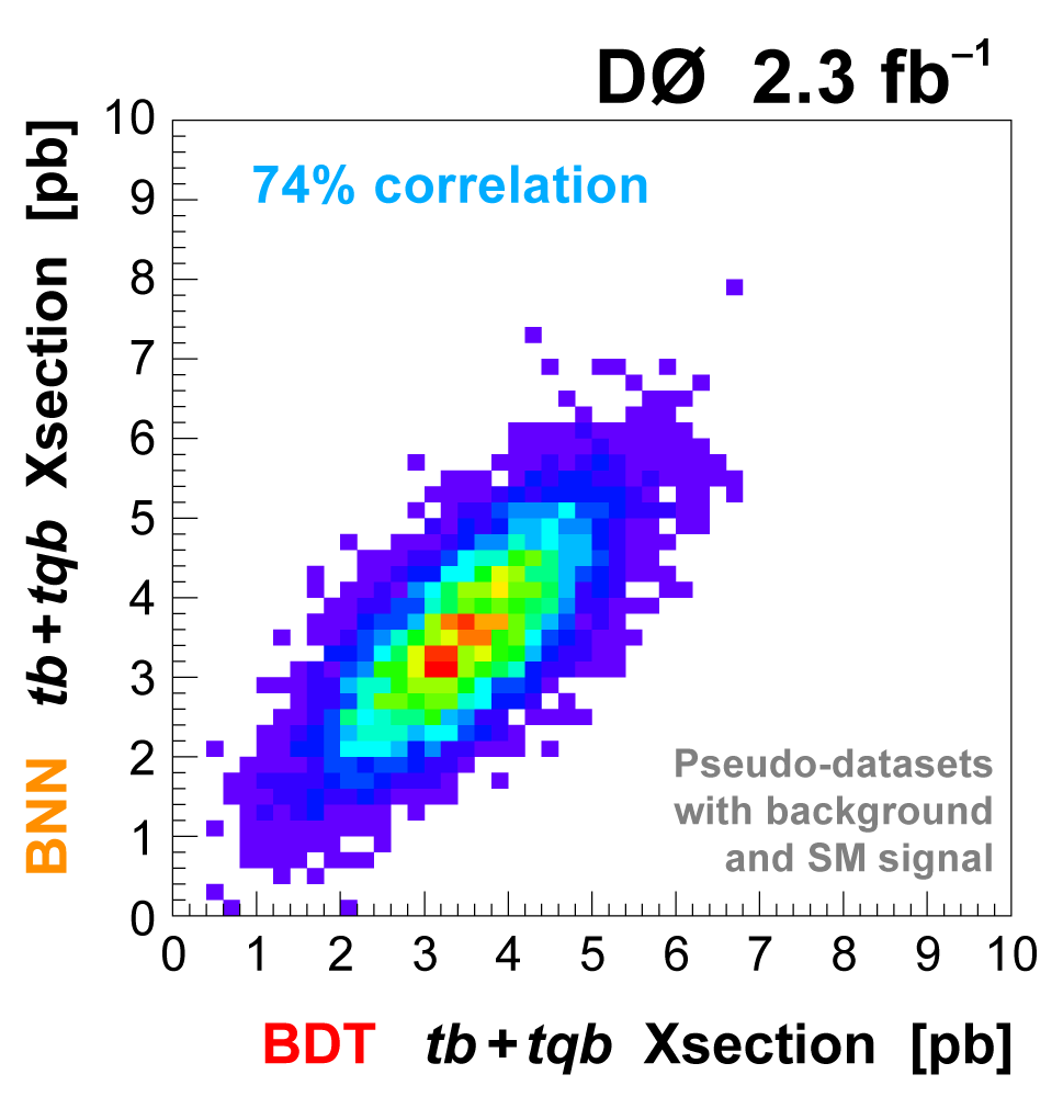
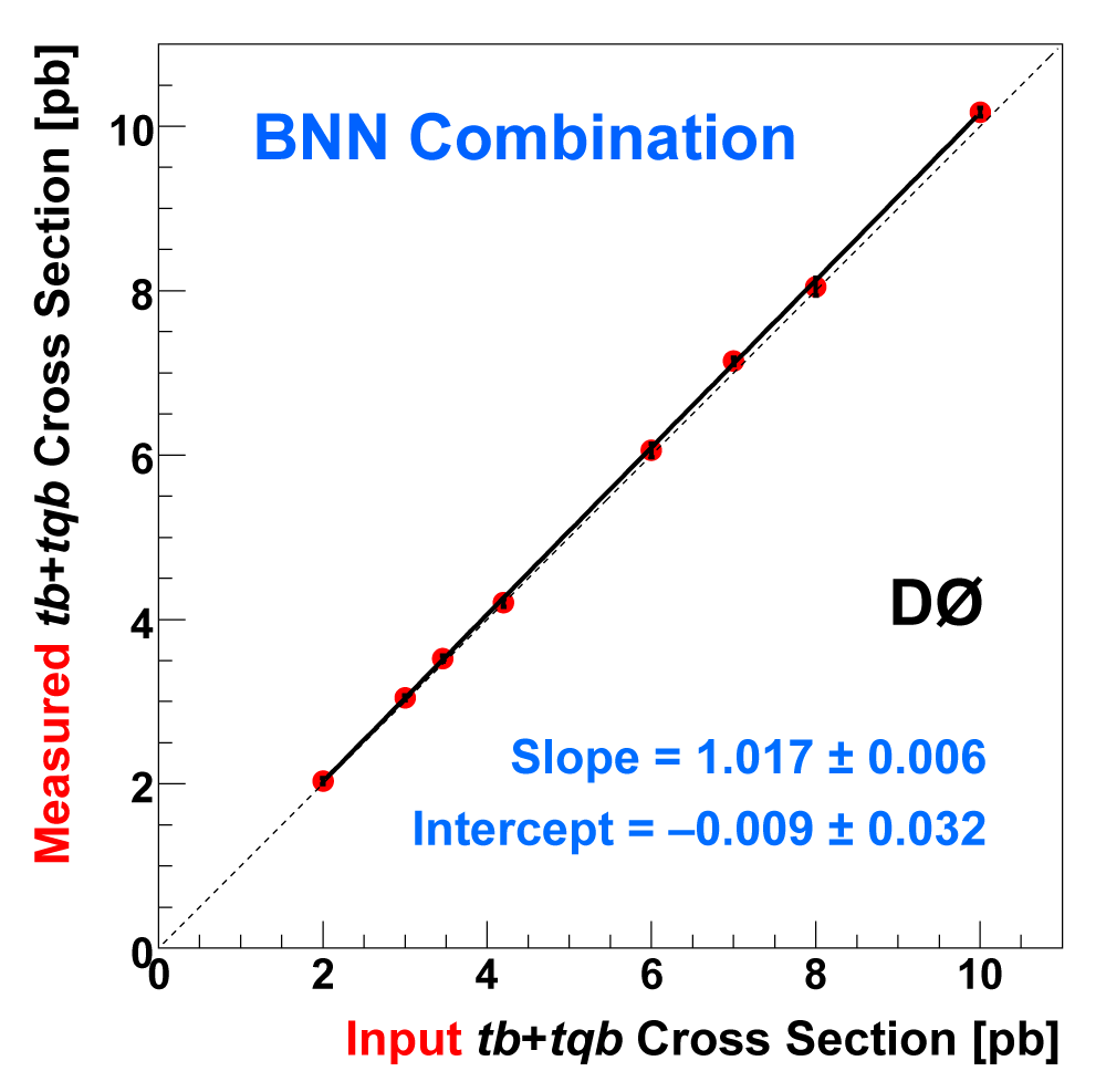
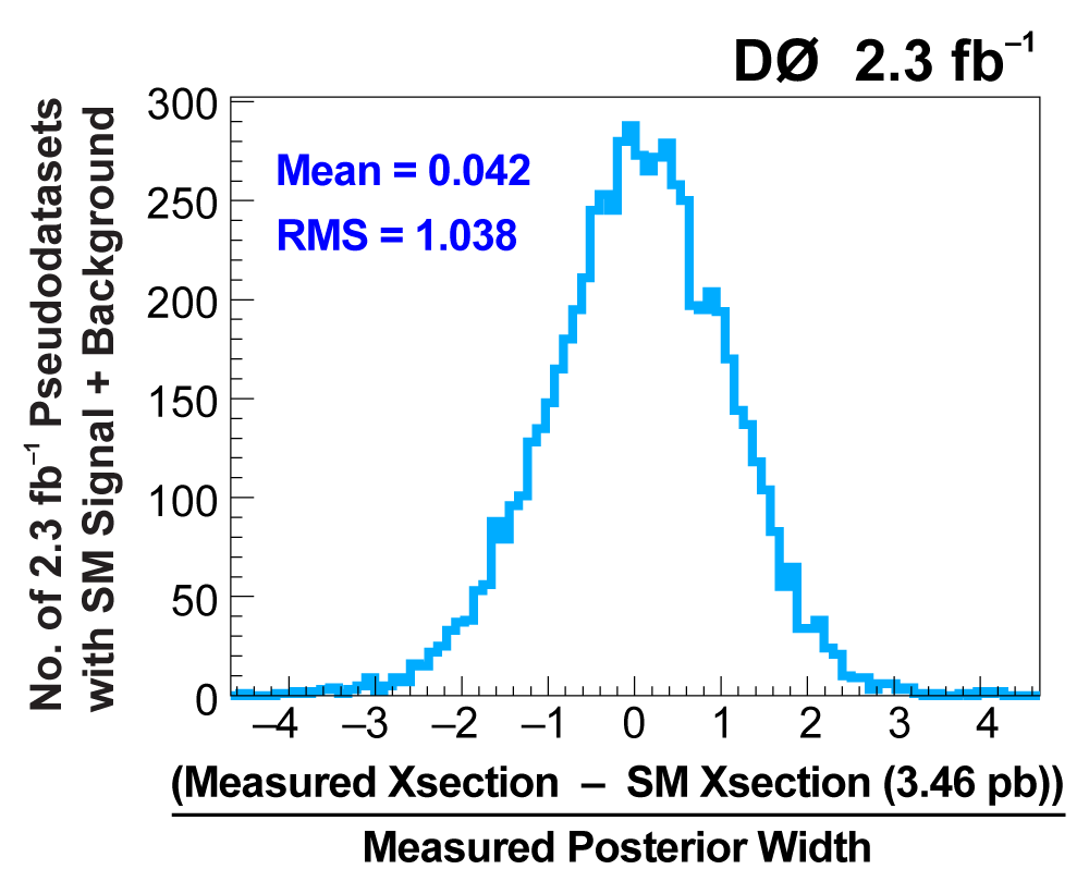
The following three plots on the right show that each of the discriminant methods is able to accurately measure the single top cross section. These plots were produced using eight ensembles of pseudo-data. Each pseudo-dataset contains signal and background events and their uncertainties that model the real 2.3 fb^-1 dataset. Each ensemble contains thousands of pseudo-datasets. The difference between the samples is the cross section value chosen for the single top events. This input cross section is reproduced by each discriminant analysis, as illustrated in the left-hand plot for the boosted decision tree discriminants and the ensemble with SM signal cross section.

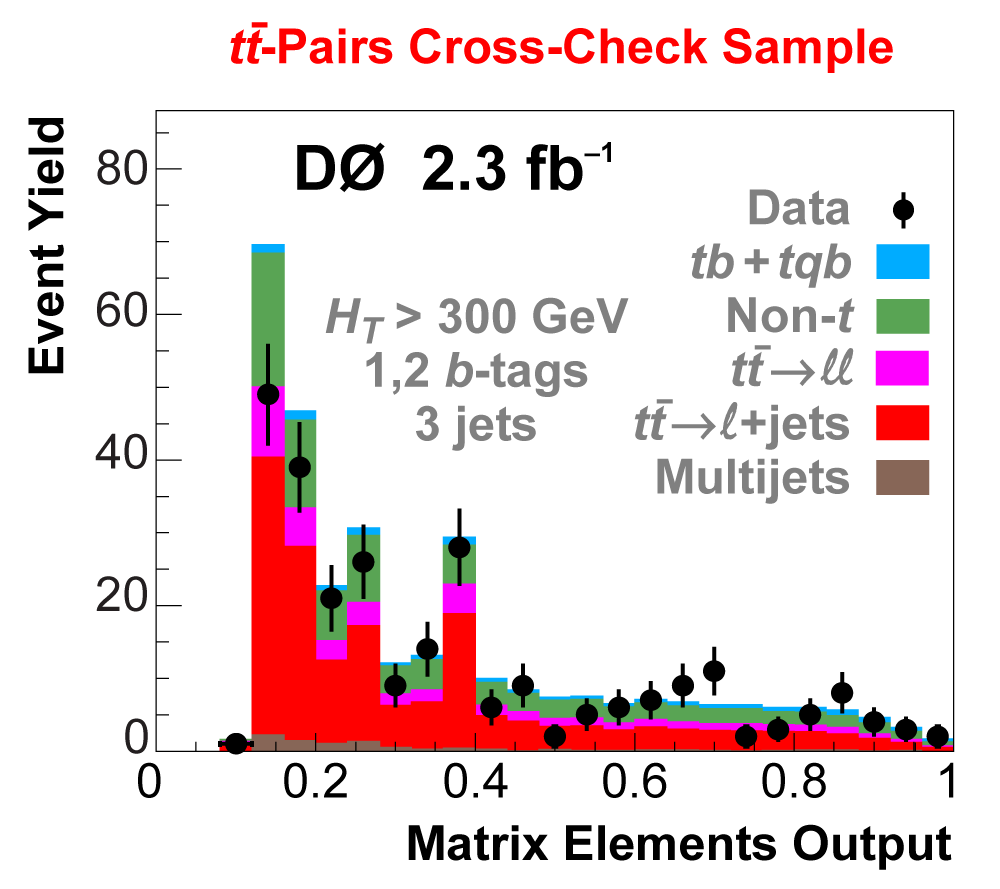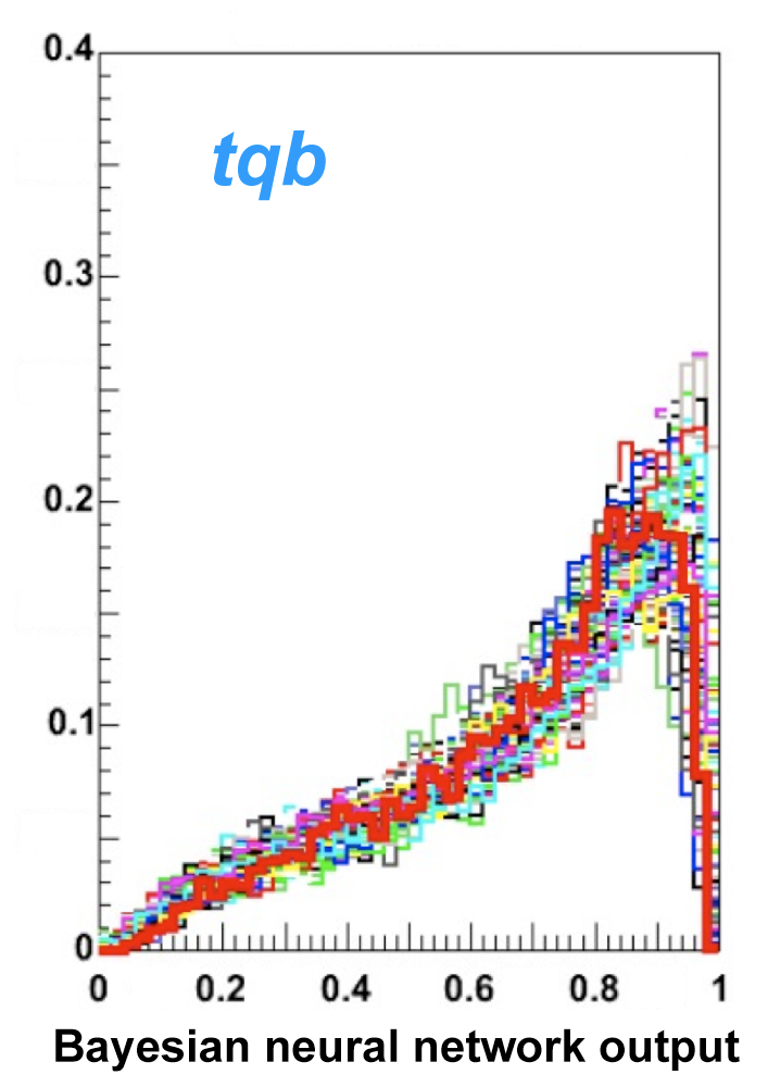
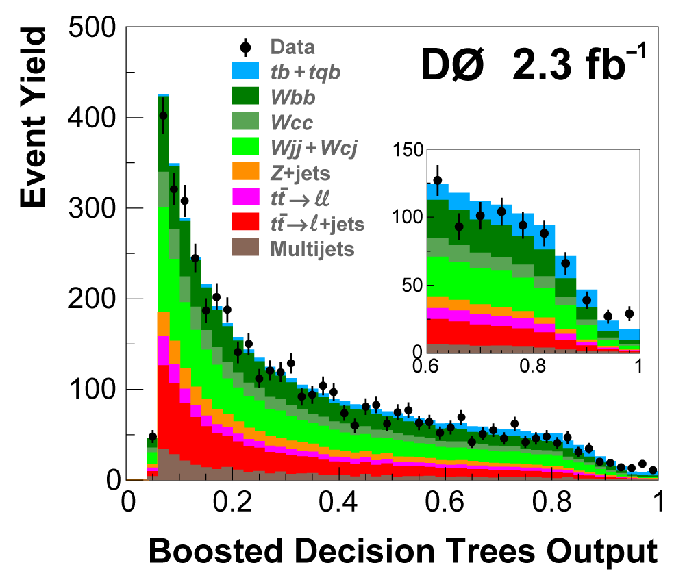
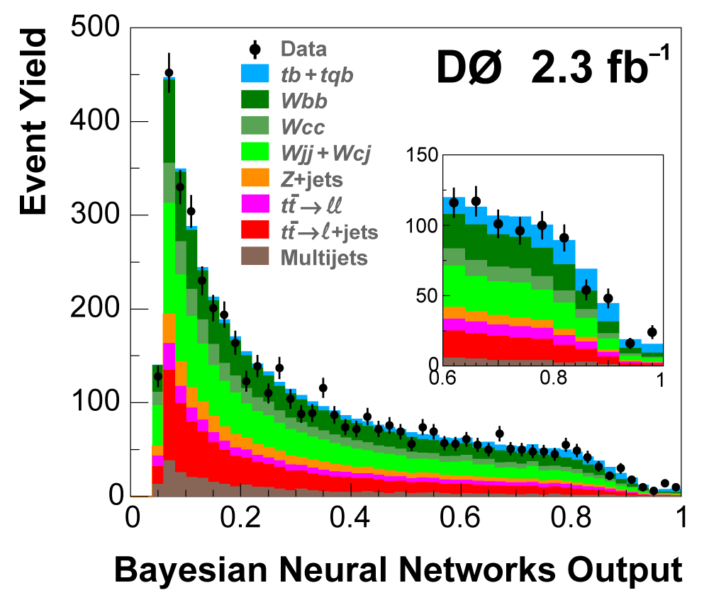
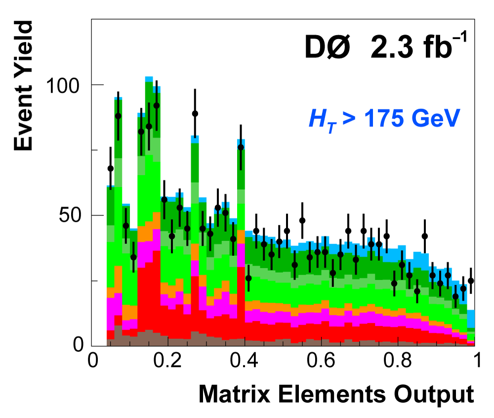
Discriminant Outputs for the Cross-Check Samples

Discriminant Outputs

The next four plots show the discriminant outputs for all analysis channels combined. The signal histogram uses the measured cross section value from each analysis. The spikes in the matrix element output distribution in the high-H_T region come from the inclusion of sixteen separate analysis channels, some of which have lower statistics than others, and so the sub-distributions span different regions of the x-axis.

Boosted decision trees discriminant output

Bayesian neural networks discriminant output

Matrix elements discriminant output, low HT

Matrix elements discriminant output, high HT

Individual Cross Section Measurements

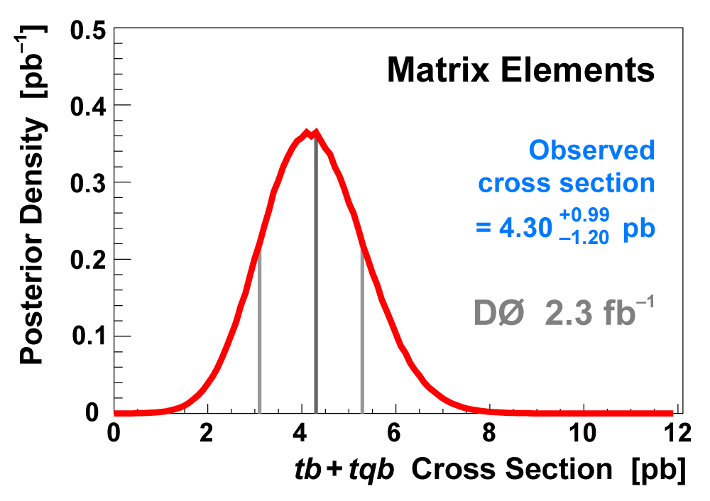
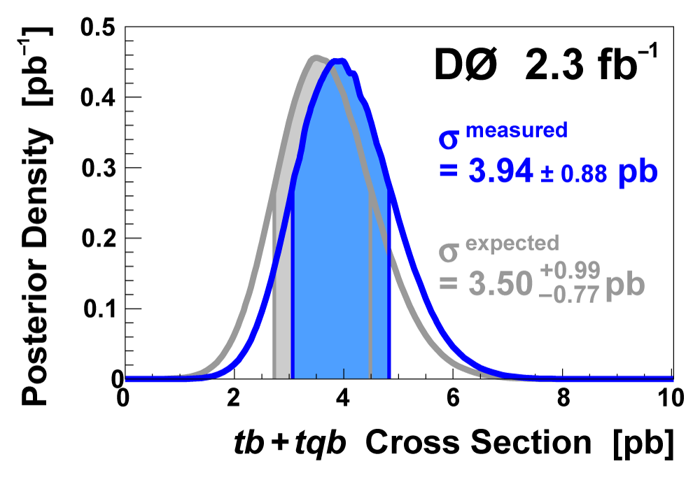
We use the discriminant output distributions (from each analysis channel separately, not all combined) to measure the single top cross section. This is a Bayesian calculation using a flat nonnegative prior for the cross section. The position of the peak of the resulting posterior density gives the cross section value, and the width of the distribution about the peak that encompasses 68% of its area gives the uncertainty (statistical and systematic components combined). The following three plots show the posterior density distributions for each discriminant method.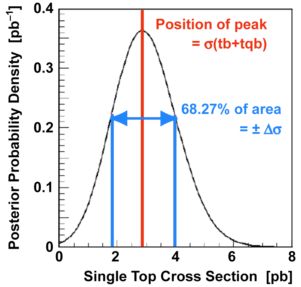

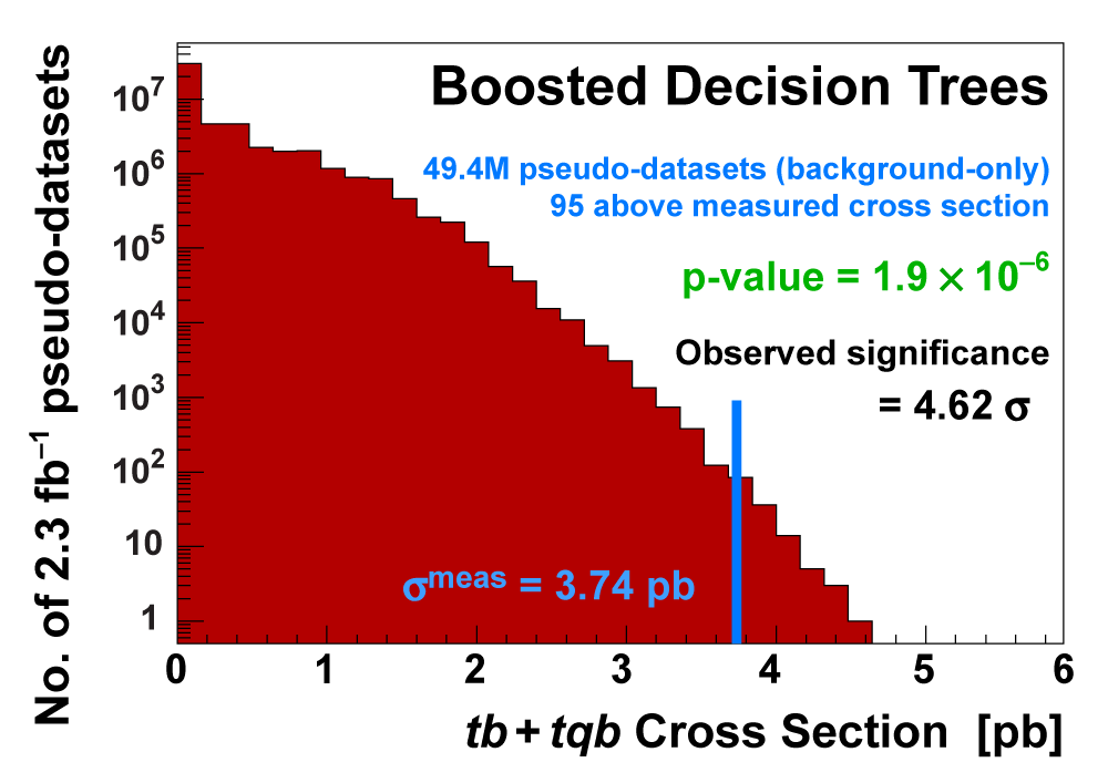
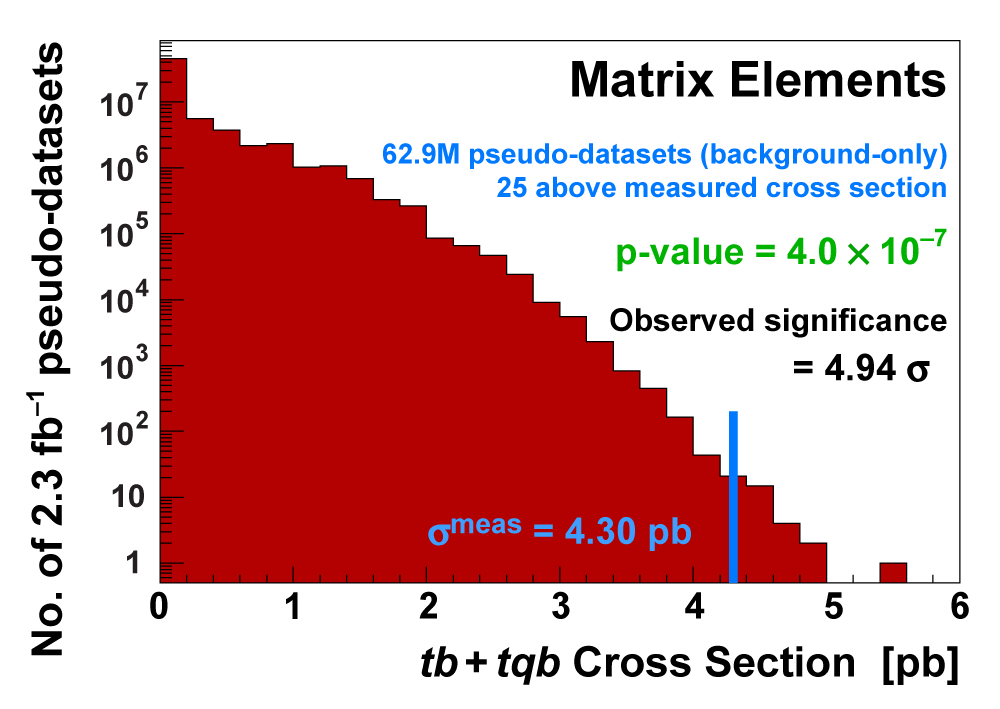
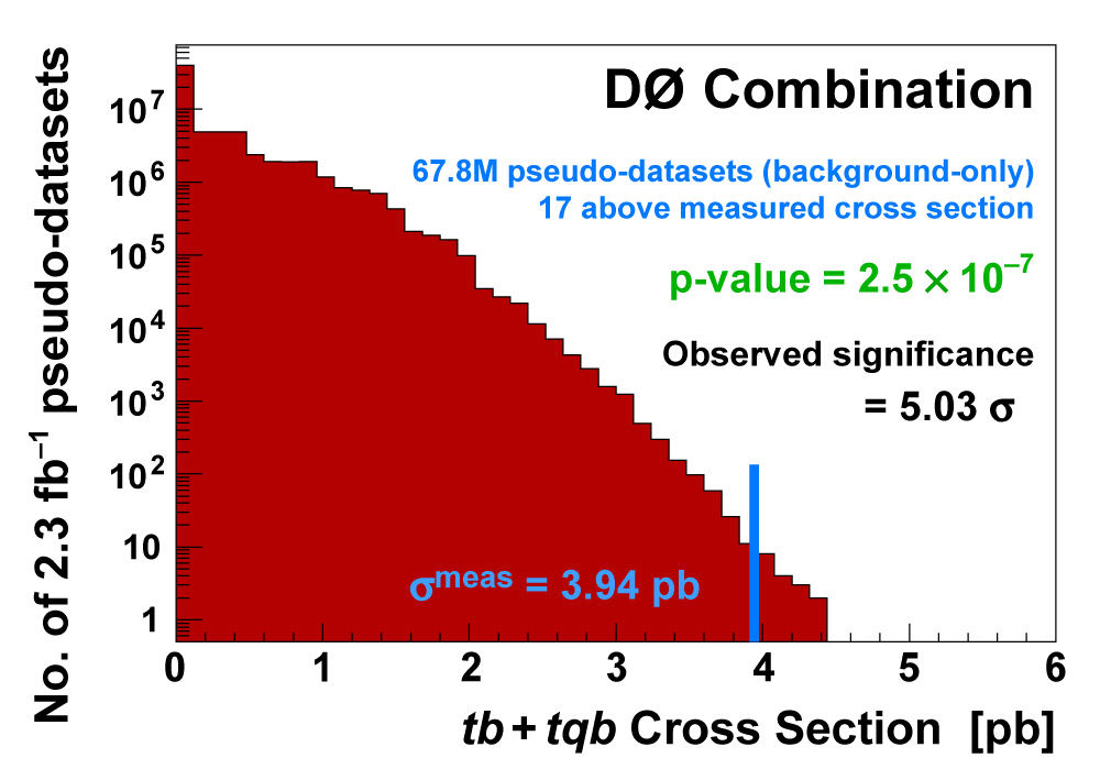
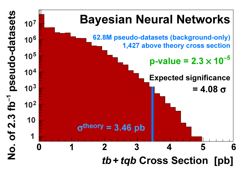
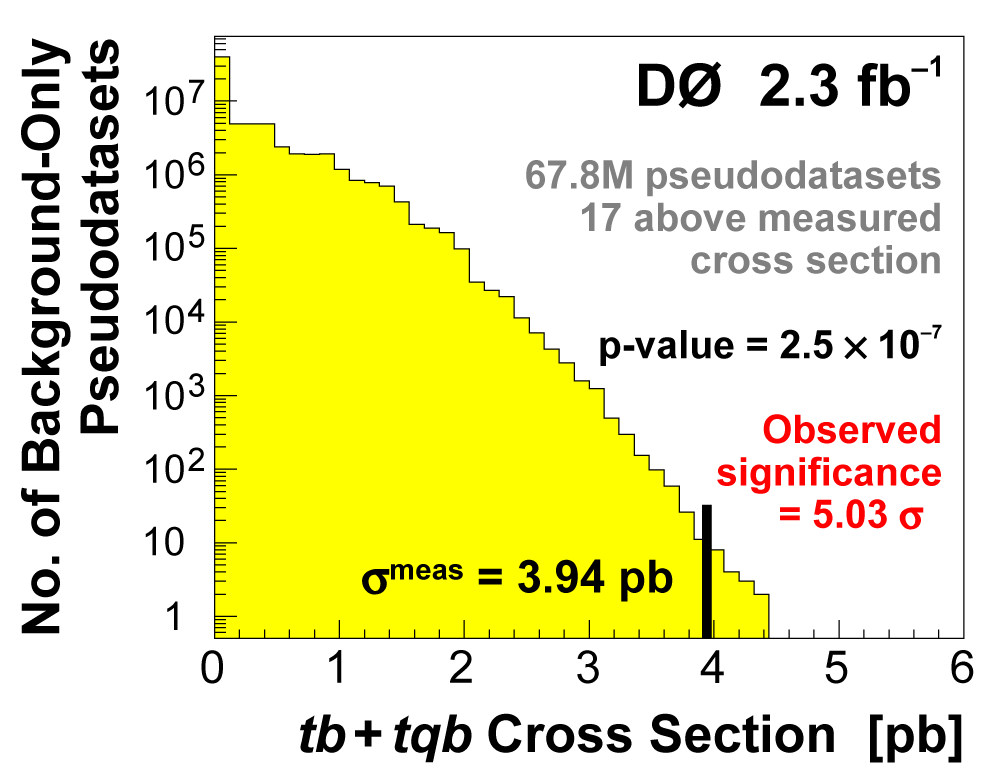
Individual Measurement Significances

We measure the probability for the background to fluctuate up and give a cross section measurement at least as large as the value we measure using a large ensemble of pseudo-datasets constructed using only background events and their uncertainties. This probability is known as the significance of the measurement. The cross section distributions measured on the pseudo-datasets are shown in the following three plots.

Individual Results Summarized

Combination of Results

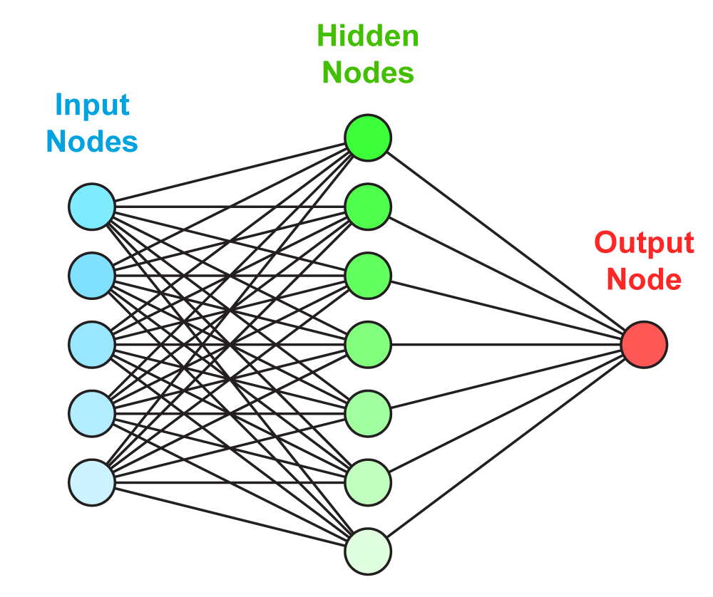
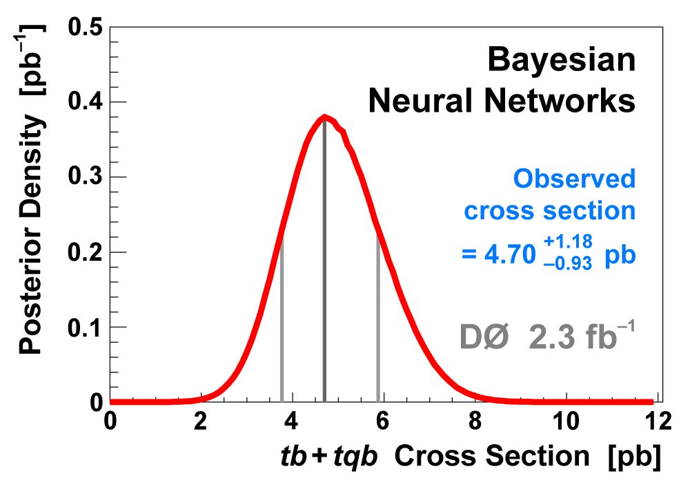
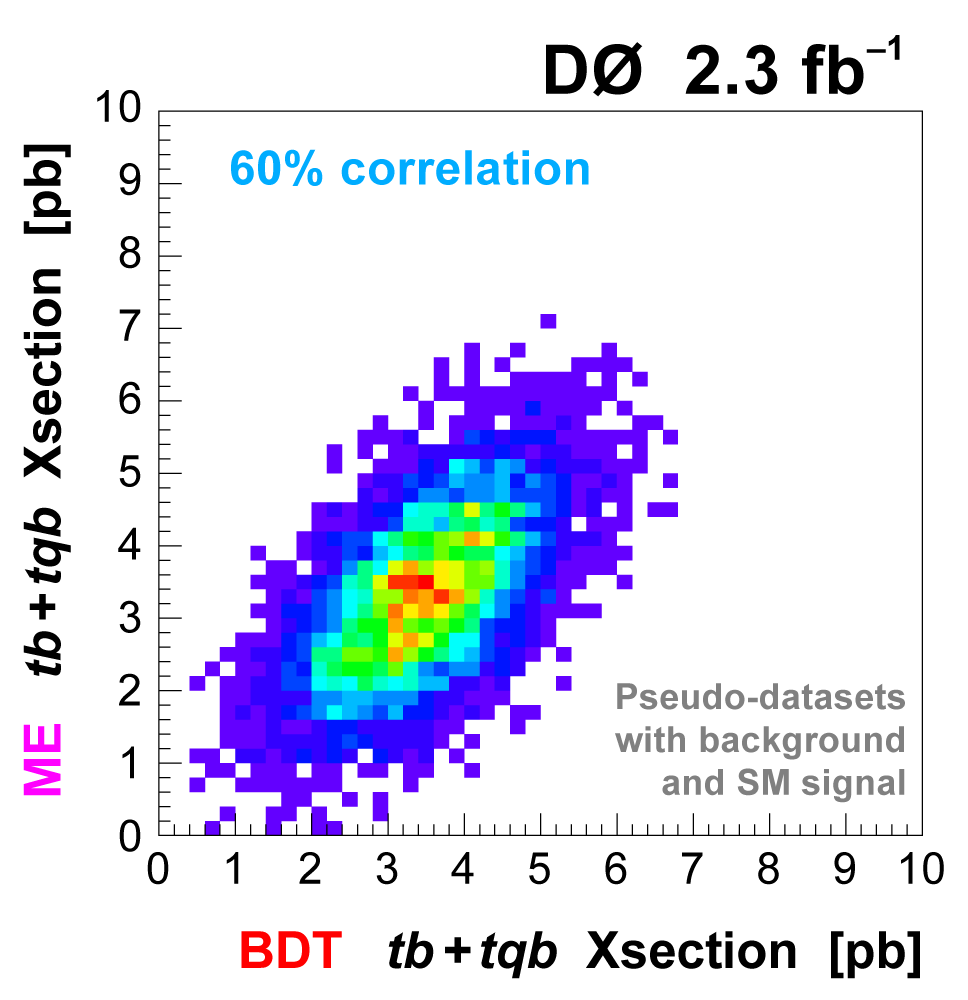
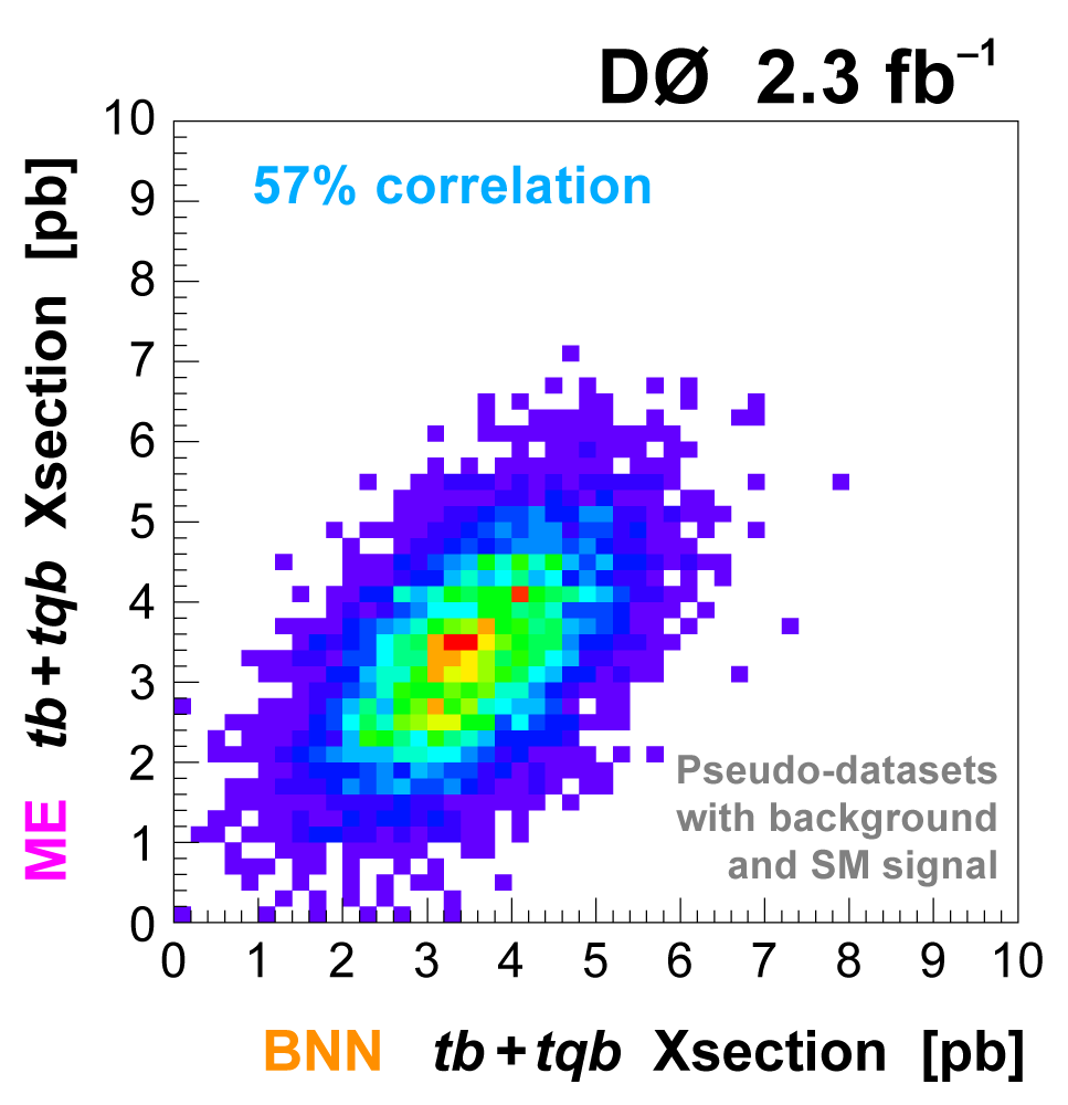
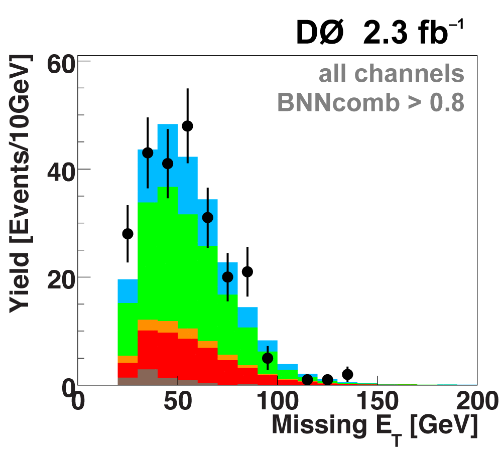
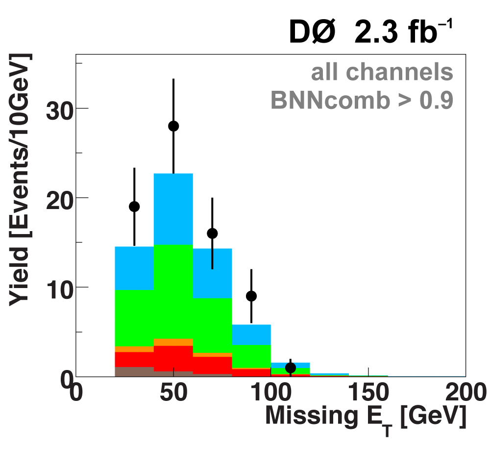
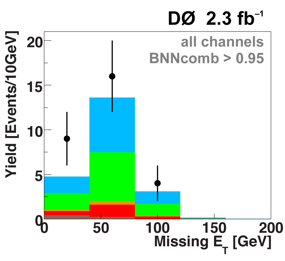
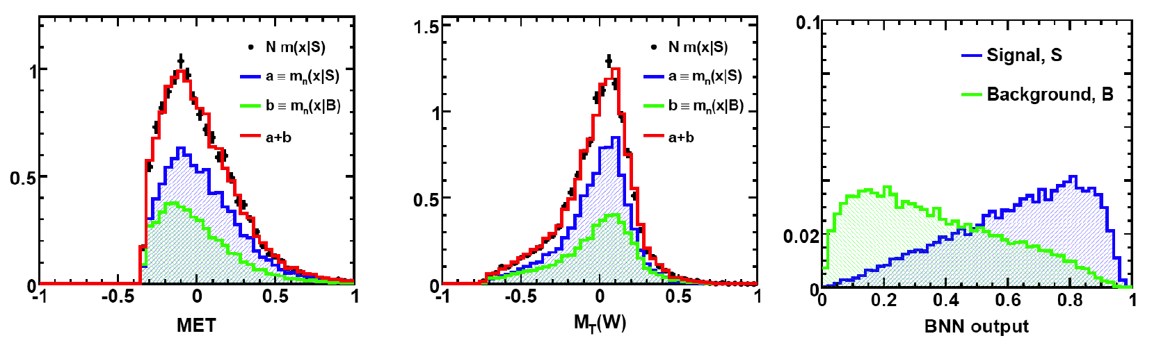
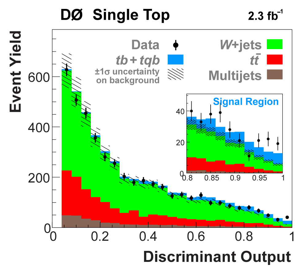
To improve the expected significance (and hopefully the measured significance) of the measurement, we combine the output distributions from the three discriminant methods, since they are not 100% correlated. We do this by using the discriminant output distributions in each analysis channel as inputs to a Bayesian neural network trained to do the combination. The BNNs have six hidden nodes. The following plots show the results of this combination.

Correlation of the Measured Cross Sections from Pairs of Discriminants

BNN analysis correlation with BDT analysis

ME analysis correlation with BDT analysis

ME analysis correlation with BNN analysis

Cross-Checks – Linearity Test and Pull Distribution

Pull distribution using SM pseudodatasets

Cross-Checks – W+jets and tt Background Models (Normalization and Shape)

W+jets cross-check sample, discriminant output

ttbar cross-check sample, discriminant output

Final Discriminant Output (bins ranked by S/B)

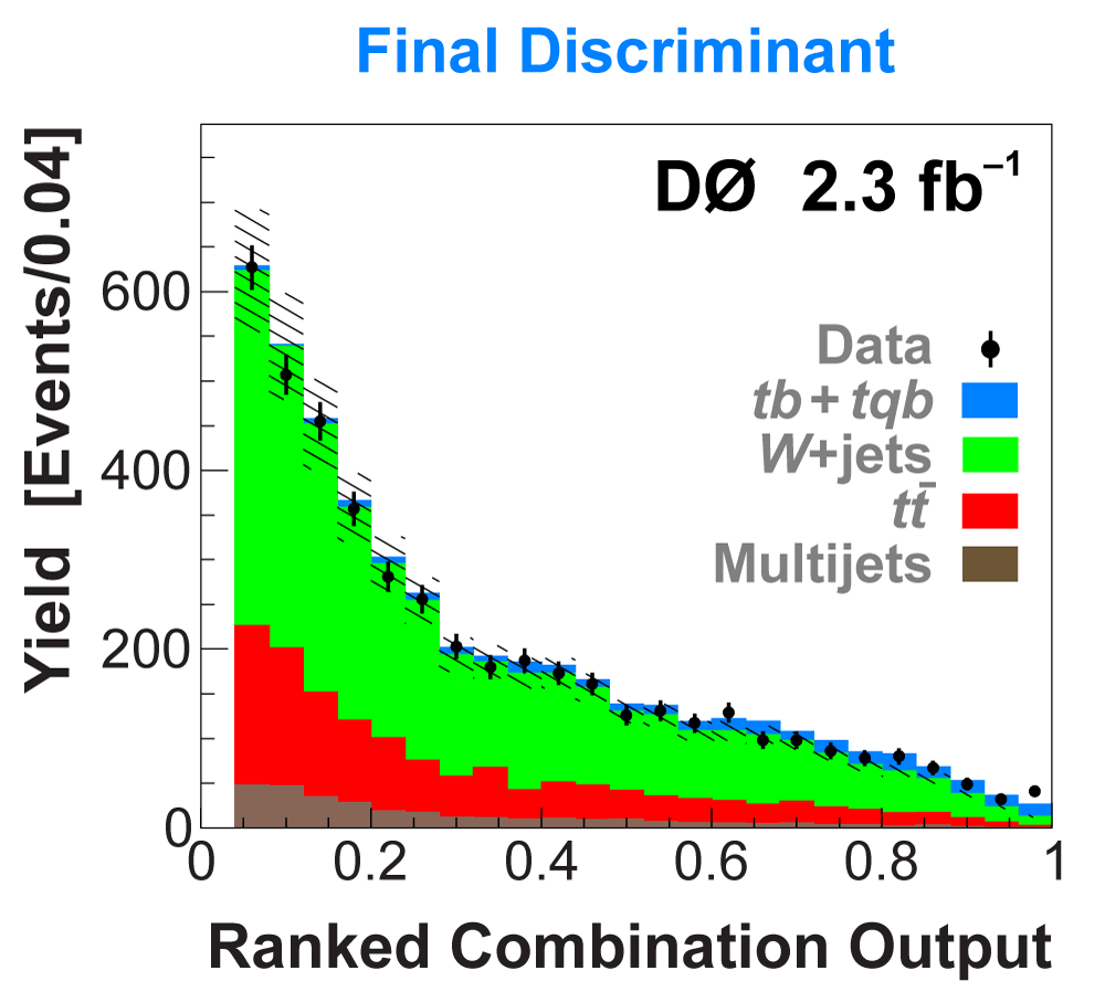
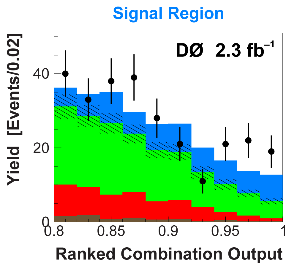
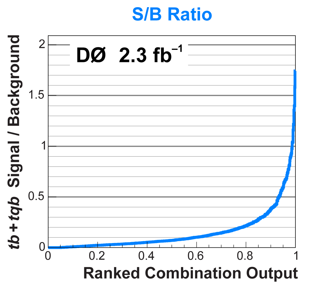
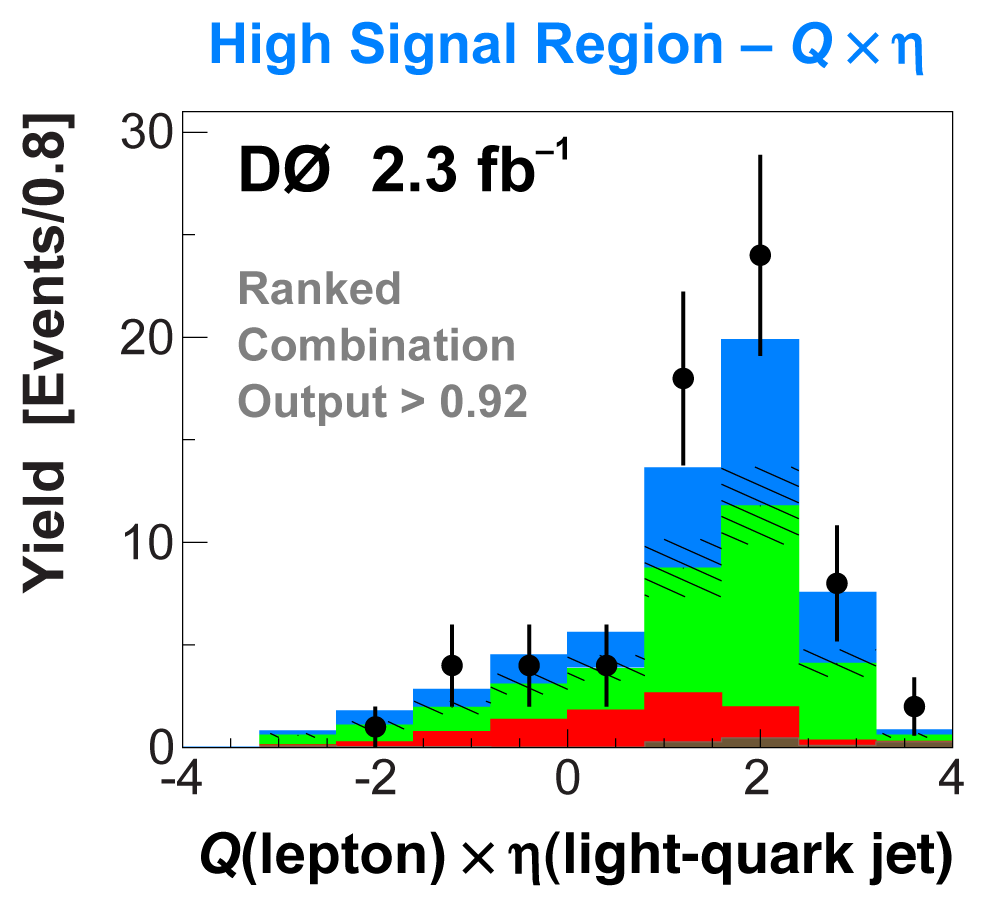
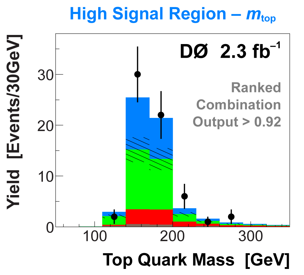
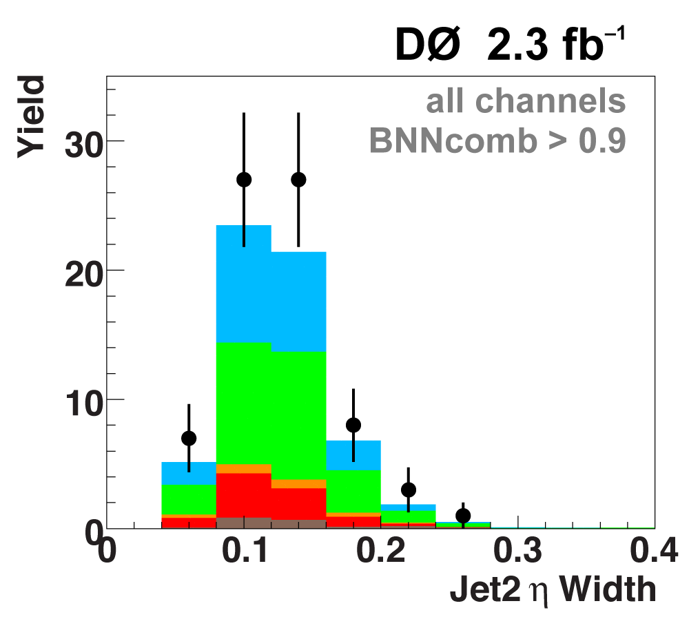
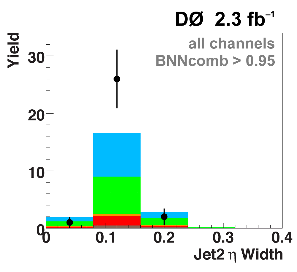
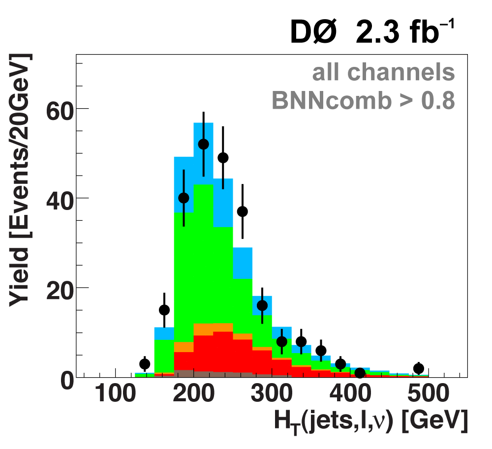
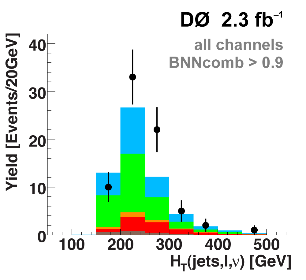
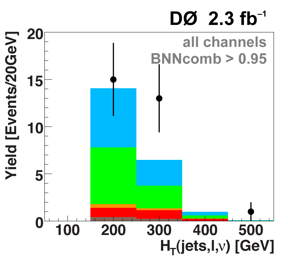
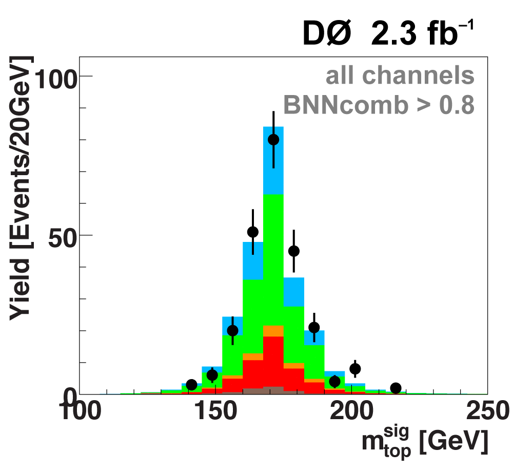
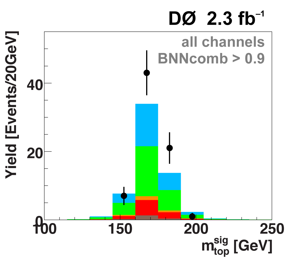
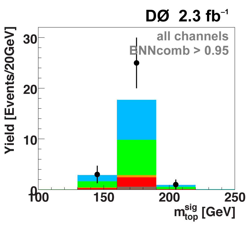
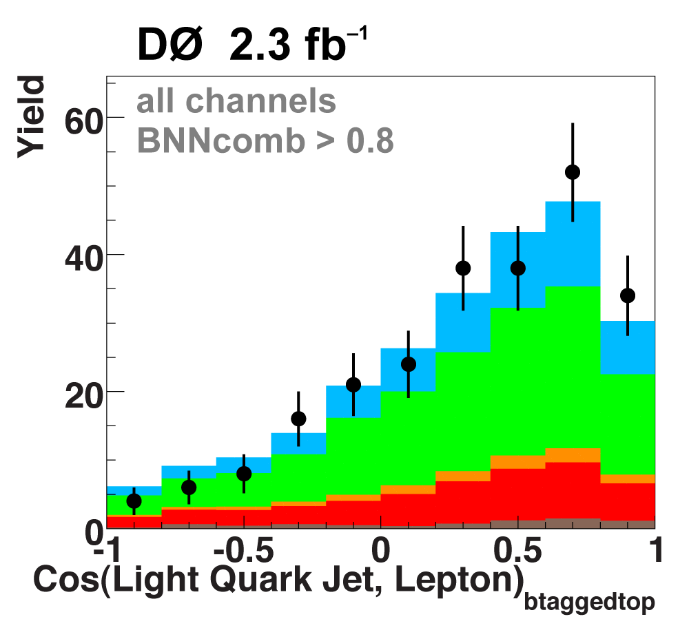
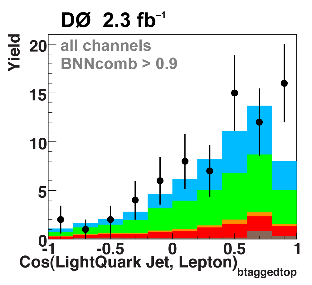
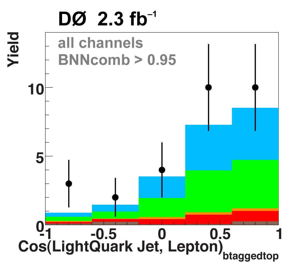
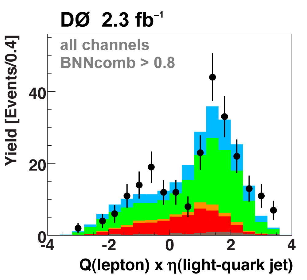
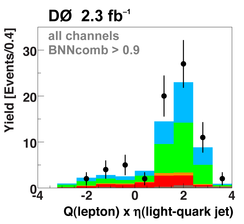
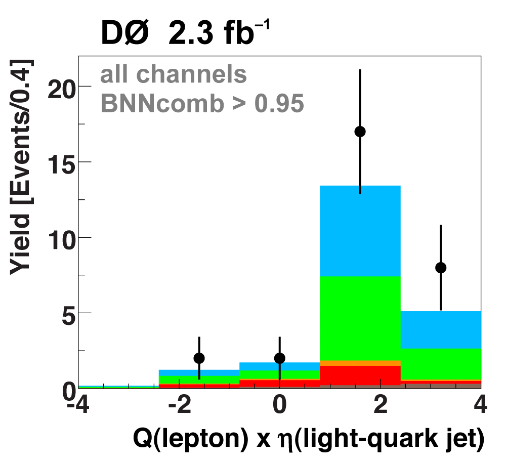
The signal histogram (shown in blue) uses the measured cross section value for normalization, for the discriminant output plots shown here and for the following two plots of sensitive variables. Please see lower down on this page for a version of the final discriminant plot with the zoomed-in high-signal region inset, suitable for review talks and proceedings papers.

Combination discriminant output, fullscale, ranked by S/B

Combination discriminant output, high end, ranked by S/B

Signal:background ratio verses ranked BNN combination output

Discriminating Variables for Events in the High Signal/Background Region

Q times Eta for high ranked combination output

Top mass for high ranked combination output

Posterior Density Distribution ("the final result") and the Significance of the Measurement

Posterior density distributions for the BNN-combination result

Cumulative Signal Plots – Full Range and Zoom of Signal Region

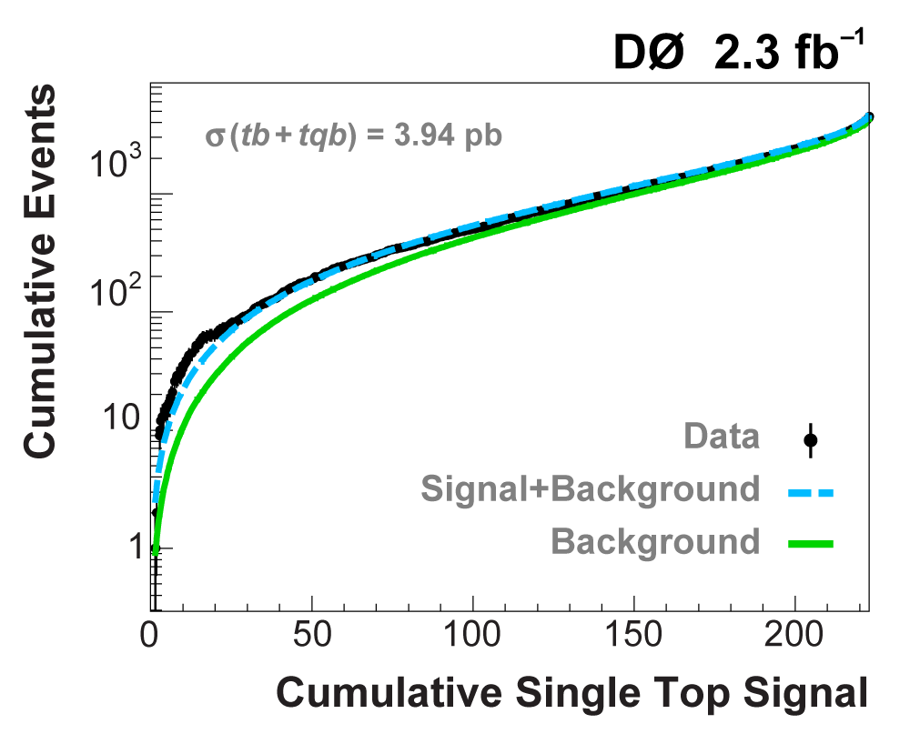
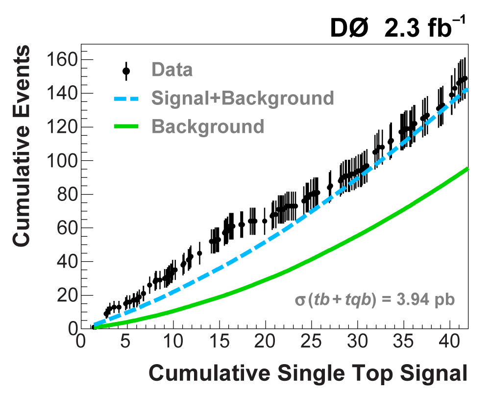
The following two plots show cumulative events versus cumulative signal (left plot is full scale, 223 signal events on the x-axis, right plot is a zoom-in of the high-signal region); the format has been developed for the Higgs boson search at the Tevatron. The plots provide an interesting new way of illustrating the presence of signal in a dataset. (Of course, in the Higgs search thus far, all data points lie along the background-only (green) line, since no signal has been seen.) The plots are created starting from the discriminant output plot with bins ranked in order of signal/background (as shown above), and for each predicted signal event, starting from the highest signal/background bin and working down, the cumulative background events (green solid line), background+signal events (blue dashed line), and data events are summed. Thus every point on the lines and the data points contain the points to the left of them and they are highly correlated. If there were no signal in the data, then the data points would lie around the background prediction line. When there is signal present, the data points cluster around the background+signal prediction, as seen in these plots. If there were not much signal predicted in the data, then the two lines would be very close together and the data could not tell the predictions apart. The plots clearly show that the data is incompatible with the background-only prediction and consistent with background+signal.

Cumulative total events versus cumulative predicted signal, full scale log plot

Cumulative total events versus cumulative predicted signal, best S:B region linear plot

In addition to the combination using a Bayesian neural network, we also combine the three sets of results using the Best Linear Unbiased Estimate (BLUE) method. This forms a valuable cross-check of the final result. Calculation of the significance of this result is in progress.

Signal Plots

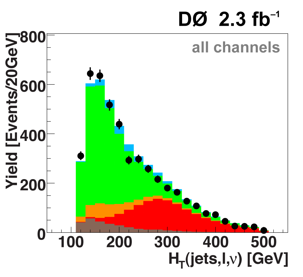
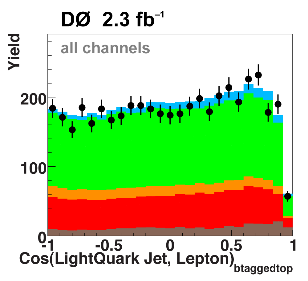
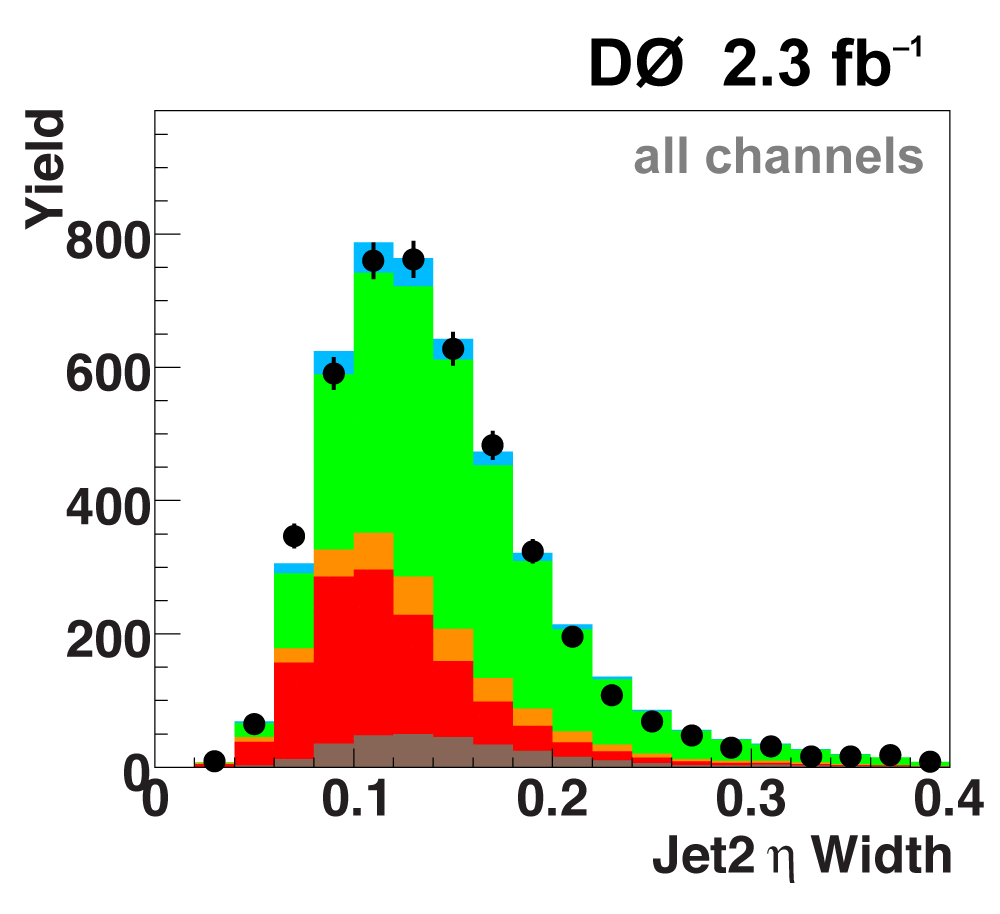
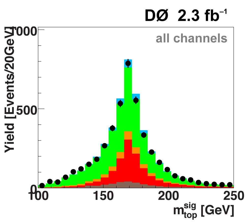
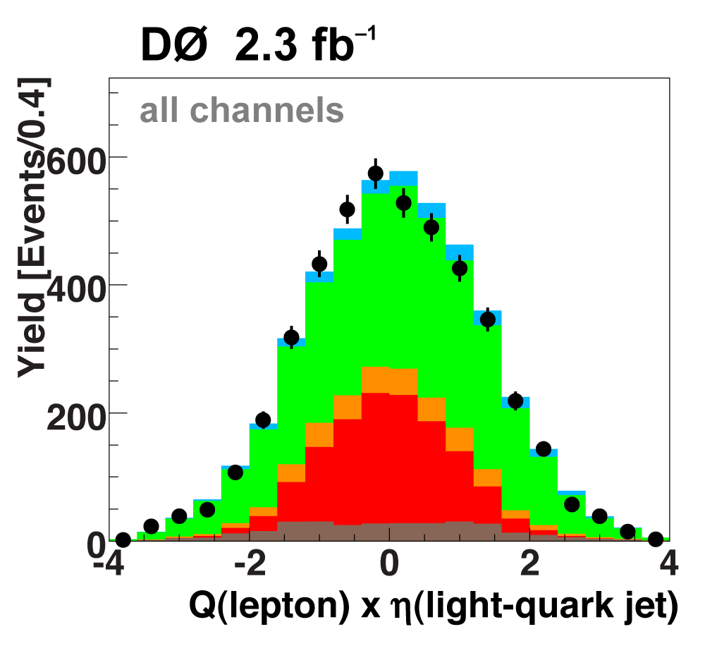
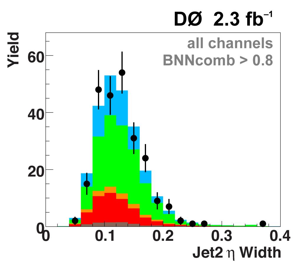
The following plots show an example discriminating variable from each category:

Object kinematics:	Missing transverse energy
Event kinematics:	Total transverse energy
Jet reconstruction:	Second jet width eta
Top quark reconstruction:	Top mass with smallest (best) significance
Angular correlations:	Cosine of the angle between the lepton and the highest p_T untagged jet in the b-tagged top mass rest frame
Object kinematics:	Charge of lepton times pseudorapidity of leading untagged jet

after progressively tighter cuts on the output of the BNN-combination discriminant. The signal:background ratio increases as the cut is tightened.
The signal histogram (shown in blue) uses the measured cross section value for normalization.

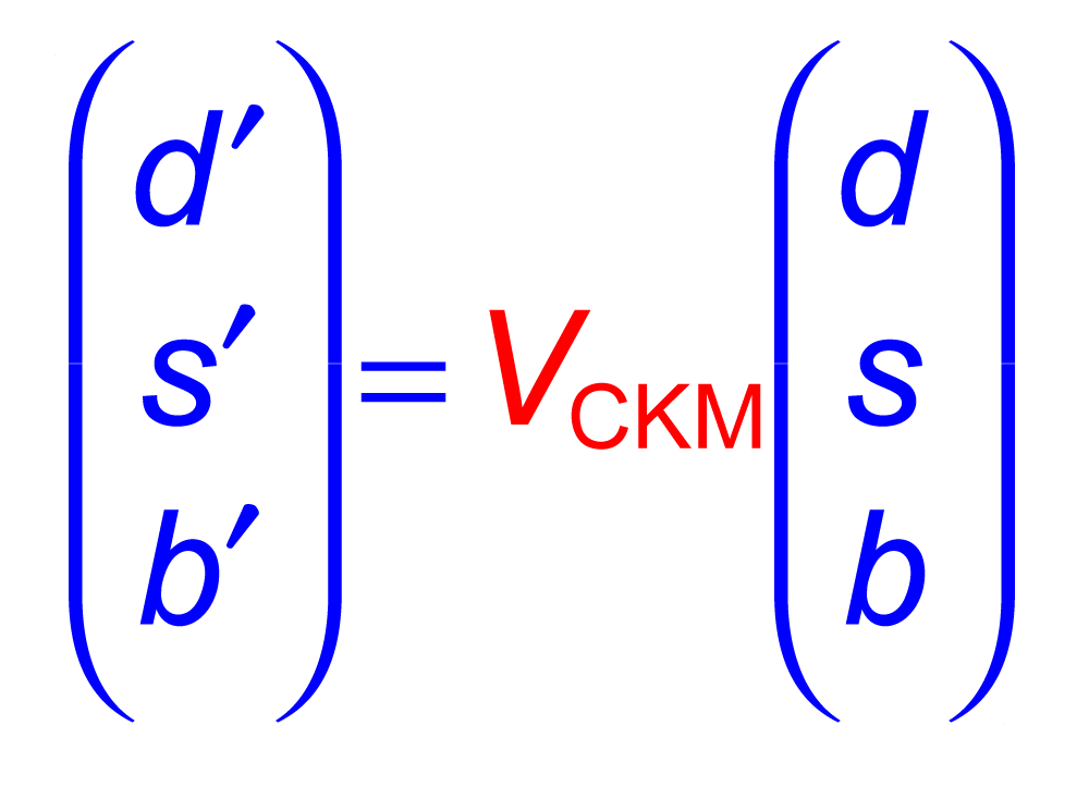
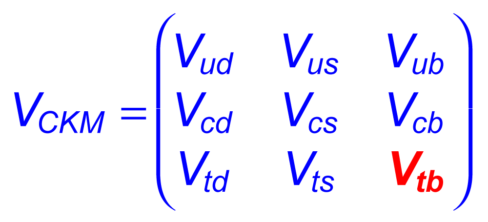
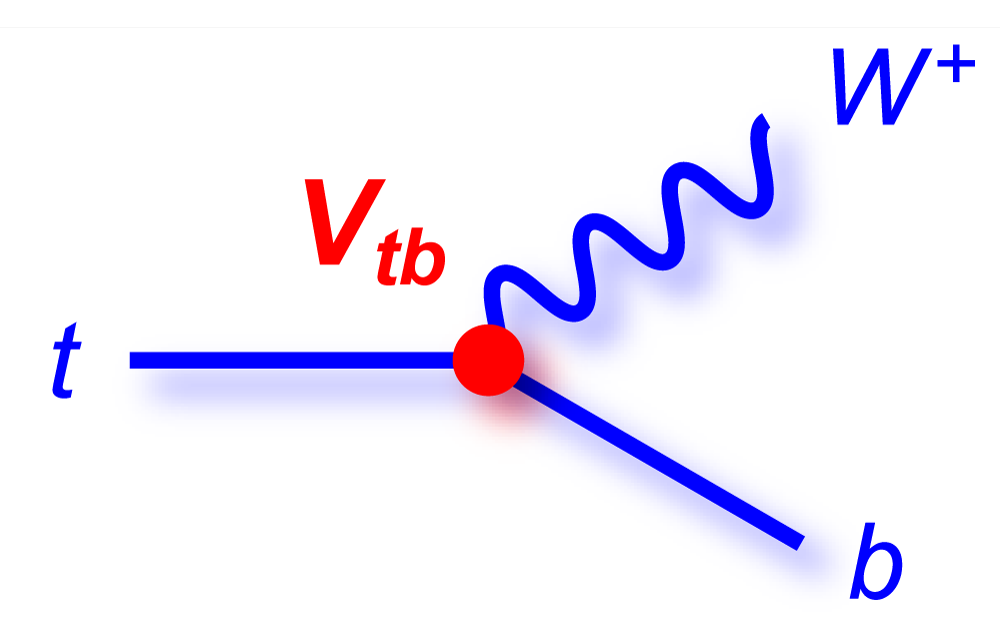
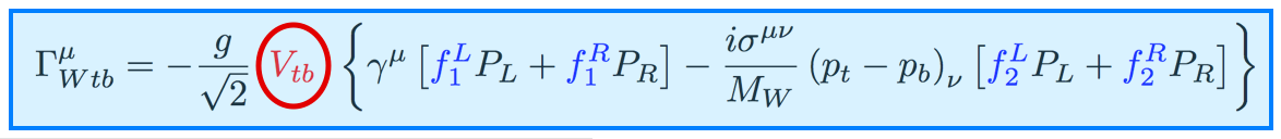
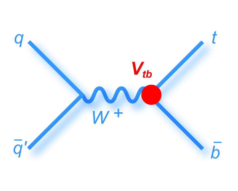
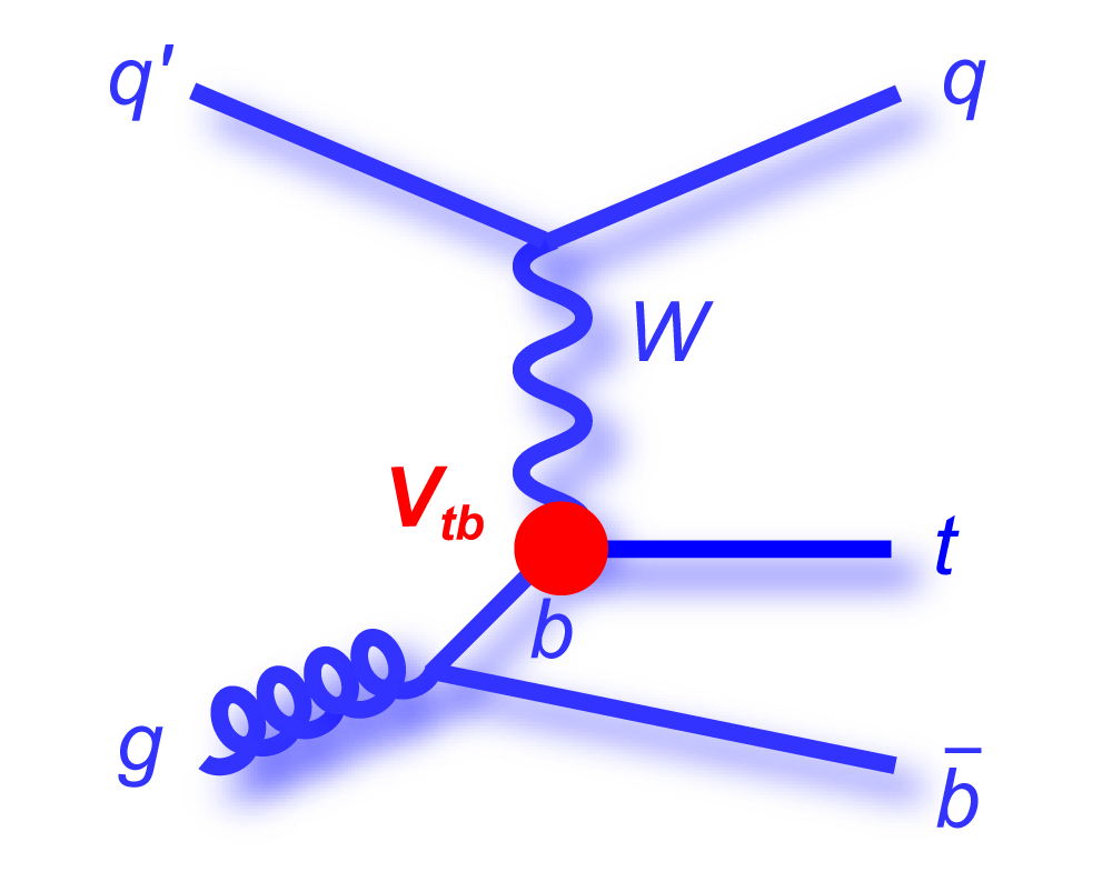
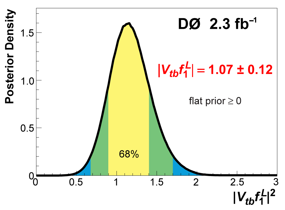
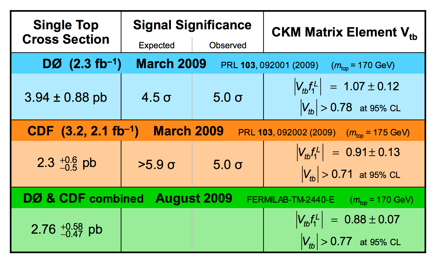
Color key for single top plots (simplified)

CKM Matrix Element |V_tb|

The Cabibbo-Kobayashi-Maskawa matrix describes the mixing between quarks to get from the strong-interaction eigenstates to the weak-interaction ones. The term relating top quarks to bottom quarks is known as V_tb. The single top quark production cross section is proportional to |V_tb|² and can thus be used to measure the amplitude of V_tb. To make this measurement, we assume the standard model for top quark decay (i.e., mostly to Wb and not much to Wd or Ws), and that the Wtb coupling is left-handed and CP-conserving. We do not assume there are exactly three quark generations for this measurement. The following two plots show our results, first for when the strength of the left-handed scalar coupling f₁^L is not constrained, and second for when it is set equal to one.

Additional uncertainties used for the Vtb measurement

feynman diagram of tb showing Wtb coupling

feynman diagram of tqb showing Wtb coupling

Vtb^2 posterior plot, no upper limit on prior

Vtb^2 posterior plot, prior less than one

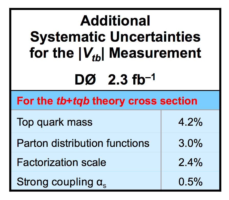
Because the uncertainty of ±0.12 on the result |V_tbf₁^L| = 1.07 ± 0.12 is determined from the width of the posterior density distribution, as shown in the left-hand plot above, it includes all components: statistics, systematics, and theory.

Observation Summary

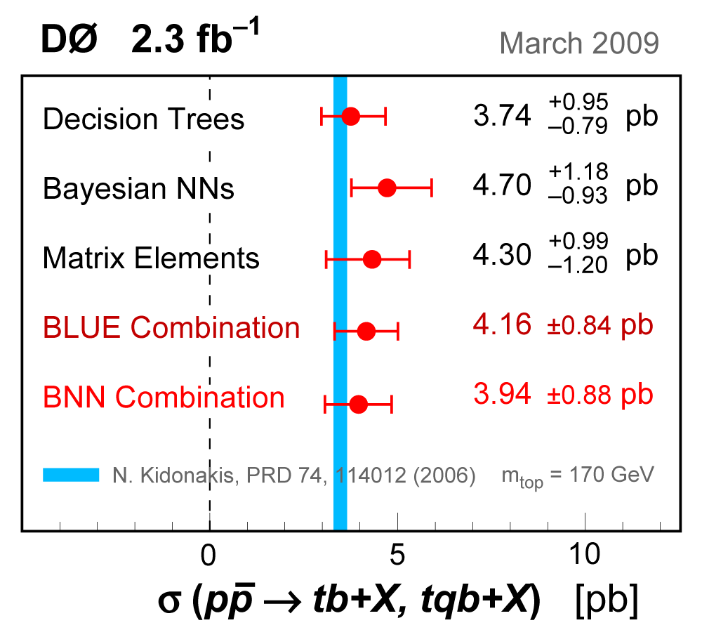
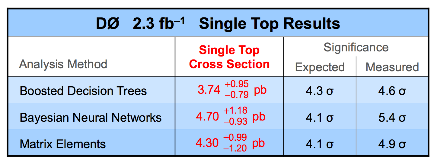
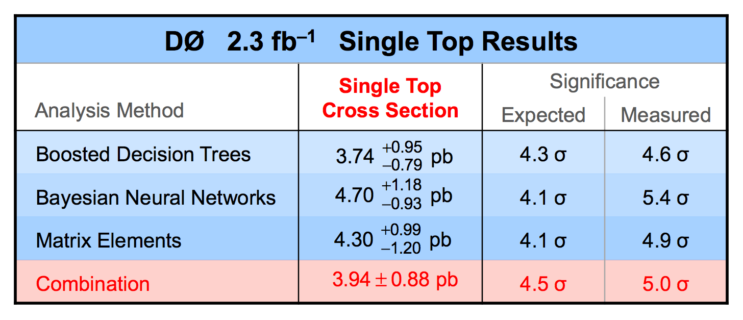
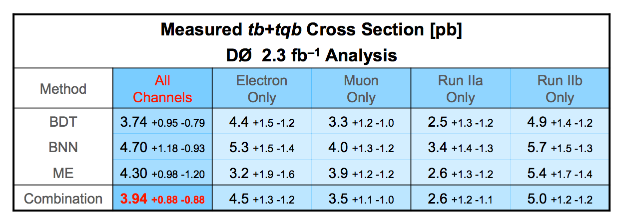
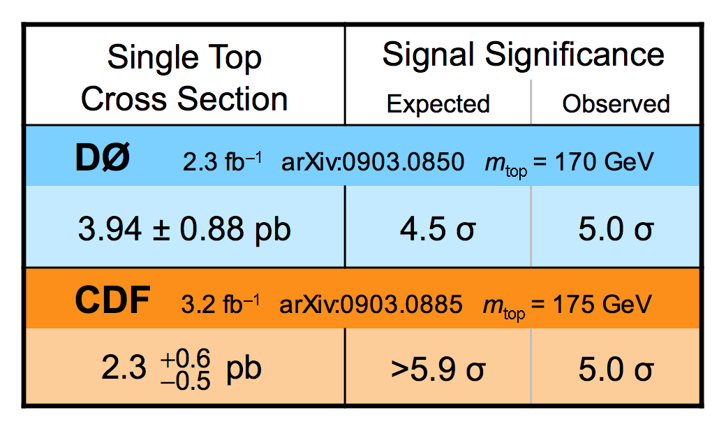
We have measured the single top quark production cross section using 2.3 fb^-1 of data at the DØ experiment. The cross section for the combined tb+tqb channels is 3.94 ± 0.88 pb. Our result provides an improved direct measurement of the amplitude of the CKM quark mixing matrix element V_tb. The measured single top quark signal corresponds to an excess over the predicted background with a p-value of 2.5 × 10^-7, which is equivalent to a significance of 5.0 standard deviations – this is the first observation of single top quark production.

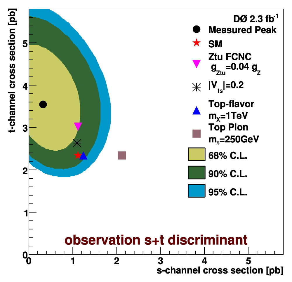
Results from the three methods and their combination

t-Channel versus s-Channel Plot

The following plots shows the posterior probability density using the final s+t channel discriminant from this analysis, as a function of the t-channel and s-channel cross sections in contours of equal probability density. Also shown are the measured cross section, SM expectation, and several representative new physics scenarios:

Flavor-changing neutral currents with a Z boson coupling to the top and up quarks with a strength of 4% of the SM coupling
4-quark-generations scenario with CKM matrix element V_ts = 0.2
Top-flavor model with new heavy bosons at a scale m_X = 1 TeV
Top-color model with a tb bound state ("top pion") with a mass of m_π = 250 GeV

from T.M.P. Tait and C.-P. Yuan, Phys. Rev. D 63, 014018 (2001) and J. Alwall et al., Eur. Phys. J. C 49, 791 (2007).

s-channel and t-channel posterior 2d plot

Talks

• Les Rencontres de Physique de la Vallée d'Aoste	DØ & CDF results	Gustavo Otero y Garzon, Universidad de Buenos Aires	March 2009
• Fermilab Joint Experimental-Theoretical Seminar	DØ results	Cecilia Gerber, University of Illinois, Chicago	March 2009
• Rencontres de Moriond: QCD and Hadronic Interactions	DØ & CDF results	Dag Gillberg, Simon Fraser University	March 2009
• HEP seminar, SLAC	DØ results	Meenakshi Narain, Brown University	March 2009
• American Physical Society April Meeting, Denver	Poster of DØ results	Ann Heinson, Cecilia Gerber, Reinhard Schwienhorst	May 2009
• American Physical Society April Meeting	DØ & CDF results	Lisa Shabalina, Georg-August-Universität Göttingen	May 2009
• American Physical Society April Meeting	DØ BDT result	Ann Heinson, University of California, Riverside	May 2009
• American Physical Society April Meeting	DØ ME result	Monica Pangilinan, Brown University	May 2009
• American Physical Society April Meeting	DØ BNN result	Cecilia Gerber, University of Illinois, Chicago	May 2009
• Madison Phenomenology Symposium	DØ results	Monica Pangilinan, Brown University	May 2009
• HEP seminar, Brookhaven	DØ results	Shabnam Jabeen, Boston University	May 2009
• HEP seminar, Bern	DØ results	Reinhard Schwienhorst, Michigan State University	May 2009
• International Conference on Supersymmetry, Boston	DØ results	Liang Li, University of California, Riverside	June 2009
• Rencontres de Blois: Windows on the Universe	DØ & CDF results	Ann Heinson, University of California, Riverside	June 2009
• Europhysics Conference on HEP, Krakow	DØ results	Reinhard Schwienhorst, Michigan State University	July 2009
• APS Division of Particles and Fields Meeting, Detroit	DØ results	Cecilia Gerber, University of Illinois, Chicago	July 2009